Dskyz (DAFE) AI Adaptive Regime - Beginners VersionDskyz (DAFE) AI Adaptive Regime - Pro: Revolutionizing Trading for All
Introduction
In the fast-paced world of financial markets, traders need tools that can keep up with ever-changing conditions while remaining accessible. The Dskyz (DAFE) AI Adaptive Regime - Pro is a groundbreaking TradingView strategy that delivers advanced, AI-driven trading capabilities to everyday traders. Available on TradingView (TradingView Scripts), this Pine Script strategy combines sophisticated market analysis with user-friendly features, making it a standout choice for both novice and experienced traders.
Core Functionality
The strategy is built to adapt to different market regimes—trending, ranging, volatile, or quiet—using a robust set of technical indicators, including:
Moving Averages (MA): Fast and slow EMAs to detect trend direction.
Average True Range (ATR): For dynamic stop-loss and volatility assessment.
Relative Strength Index (RSI) and MACD: Multi-timeframe confirmation of momentum and trend.
Average Directional Index (ADX): To identify trending markets.
Bollinger Bands: For assessing volatility and range conditions.
Candlestick Patterns: Recognizes patterns like bullish engulfing, hammer, and double bottoms, confirmed by volume spikes.
It generates buy and sell signals based on a scoring system that weighs these indicators, ensuring trades align with the current market environment. The strategy also includes dynamic risk management with ATR-based stops and trailing stops, as well as performance tracking to optimize future trades.
What Sets It Apart
The Dskyz (DAFE) AI Adaptive Regime - Pro distinguishes itself from other TradingView strategies through several unique features, which we compare to common alternatives below:
| Feature | Dskyz (DAFE) | Typical TradingView Strategies|
|---------|-------------|------------------------------------------------------------|
| Regime Detection | Automatically identifies and adapts to **four** market regimes | Often static or limited to trend/range detection |
| Multi‑Timeframe Analysis | Uses higher‑timeframe RSI/MACD for confirmation | Rarely incorporates multi‑timeframe data |
| Pattern Recognition | Detects candlestick patterns **with volume confirmation** | Limited or no pattern recognition |
| Dynamic Risk Management | ATR‑based stops and trailing stops | Often uses fixed stops or basic risk rules |
| Performance Tracking | Adjusts thresholds based on past performance | Typically static parameters |
| Beginner‑Friendly Presets | Aggressive, Conservative, Optimized profiles | Requires manual parameter tuning |
| Visual Cues | Color‑coded backgrounds for regimes | Basic or no visual aids |
The Dskyz strategy’s ability to integrate regime detection, multi-timeframe analysis, and user-friendly presets makes it uniquely versatile and accessible, addressing the needs of everyday traders who want professional-grade tools without the complexity.
-Key Features and Benefits
[Why It’s Ideal for Everyday Traders
⚡The Dskyz (DAFE) AI Adaptive Regime - Pro democratizes advanced trading by offering professional-grade tools in an accessible package. Unlike many TradingView strategies that require deep technical knowledge or fail in changing market conditions, this strategy simplifies complex analysis while maintaining robustness. Its presets and visual aids make it easy for beginners to start, while its adaptive features and performance tracking appeal to advanced traders seeking an edge.
🔄Limitations and Considerations
Market Dependency: Performance varies by market and timeframe. Backtesting is essential to ensure compatibility with your trading style.
Learning Curve: While presets simplify use, understanding regimes and indicators enhances effectiveness.
No Guaranteed Profits: Like all strategies, success depends on market conditions and proper execution. The Reddit discussion highlights skepticism about TradingView strategies’ universal success (Reddit Discussion).
Instrument Specificity: Optimized for futures (e.g., ES, NQ) due to fixed tick values. Test on other instruments like stocks or forex to verify compatibility.
📌Conclusion
The Dskyz (DAFE) AI Adaptive Regime - Pro is a revolutionary TradingView strategy that empowers everyday traders with advanced, AI-driven tools. Its ability to adapt to market regimes, confirm signals across timeframes, and manage risk dynamically. sets it apart from typical strategies. By offering beginner-friendly presets and visual cues, it makes sophisticated trading accessible without sacrificing power. Whether you’re a novice looking to trade smarter or a pro seeking a competitive edge, this strategy is your ticket to mastering the markets. Add it to your chart, backtest it, and join the elite traders leveraging AI to dominate. Trade like a boss today! 🚀
Use it with discipline. Use it with clarity. Trade smarter.
**I will continue to release incredible strategies and indicators until I turn this into a brand or until someone offers me a contract.
-Dskyz
ابحث في النصوص البرمجية عن "the strat"

Daily Bollinger Band StrategyOverview of the Daily Bollinger Band Strategy
1. Strategy Overview and Features
This strategy is a tool for backtesting a trading method that uses Bollinger Bands. It is *not* a tool for automated trading.
1-1. Main Display Items
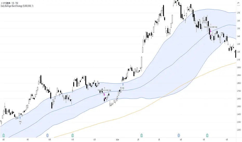
The main chart displays the Bollinger Bands and the 200-day moving average.
It also shows the entry and exit points along with the position size (in units of 100 shares).
1-2. Summary of Trading Rules
For long (buy) strategies, the trade enters when the price crosses above the +1σ line of the Bollinger Bands, aiming to ride an upward trend. The position is exited when the price crosses below the middle band.
For short (sell) strategies, the trade enters when the price crosses below the -1σ line of the Bollinger Bands, aiming to ride a downward trend. The position is exited when the price crosses above the middle band.
1-3. Strategic Enhancements
The strategy uses the slope of the 200-day moving average to determine the trend direction and enter trades accordingly. This improves the win rate and payoff ratio.
Additionally, to reduce the probability of ruin, the risk per trade is limited to 1.0% of capital, and position sizing is adjusted using ATR (a volatility indicator).
2. Trading Rules
2-1. Chart Type
Only daily charts are used.
2-2. Indicators Used
(1) Bollinger Bands** (used for entry and exit signals)
- Period: Fixed at 80 days
- Upper and lower bands: Fixed at ±1σ
(2) Moving Average** (used to determine trend direction)
- Period: Fixed at 200 days
- Trend direction is judged based on whether the difference from the previous day is positive (upward) or negative (downward)
2-3. Buy Rules
Setup:
- Price crosses above the +1σ line from below
- Both the middle band and 200-day moving average are upward sloping
Entry:
- Buy at the next day’s market open using a market order
Exit:
- If the price crosses below the middle band, sell at the next day’s open using a market order
2-4. Sell Rules
Setup:
- Price crosses below the -1σ line from above
- Both the middle band and 200-day moving average are downward sloping
Entry:
- Sell at the next day’s market open using a market order
Exit:
- If the price crosses above the middle band, buy back at the next day’s open using a market order
2-5. Risk Management Rules
- Risk per trade: 1.0% of total capital (acceptable loss = capital × 1.0%)
- Position size: Acceptable loss ÷ 2ATR (rounded down to the nearest unit of 100 shares)
2-6. Other Notes
- No brokerage fees
- No pyramiding
- No partial exits
- No reverse positions (no “stop-and-reverse” trades)
3. Strategy Parameters
The following settings can be specified:
3-1. Period Settings
- Start date: Set the start date for the backtest period
- Stop date: Set the end date for the backtest period
3-2. Display of Trend and Signals
- Show trend: When checked, the background color of the bars is light red for an uptrend and light blue for a downtrend
- Show signal: When checked, entry and exit signals are displayed (note: signals are executed at the next day’s open, so there is a one-day lag in the display)
3-3. Capital Management Settings
- Funds: Capital available for trading (in JPY)
- Risk rate: Specify what percentage of the capital to risk per trade
Settings in the “Properties” tab are not used in this strategy.
4. Backtest Results (Example)
Here are the backtest results conducted by the author:
- Target Stocks: All components of the Nikkei 225
- Test Period: January 4, 2000 – December 30, 2024
- Data Points: 12,886
- Win Rate: 33.45%
- Net Profit: ¥82,132,380
- Payoff Ratio: 2.450
- Expected Value: ¥6,373.8
- Risk Rate: 1.0%
- Probability of Ruin: 0.00%
---
デイリー・ボリンジャーバンド・ストラテジーの概要
1. ストラテジーの概要と特徴
このストラテジーは、ボリンジャーバンドを使ったトレード手法のバックテストを行うツールです。自動売買を行うツールではありません。
1-1. 主な表示項目
メインチャートにボリンジャーバンドと 200日移動平均線を表示します。
また、エントリーと手仕舞いのタイミングと数量(100株単位)も表示されます。
1-2. トレードルールの概要
買い戦略の場合、ボリンジャーバンドの +1σ 超えでエントリーして上昇トレンドに乗り、ミドルバンドを割ったら決済します。
売り戦略の場合、ボリンジャーバンドの -1σ 割りでエントリーして下降トレンドに乗り、ミドルバンドを上抜けたら決済します。
1-3. ストラテジーの工夫点
200日移動平均線の傾きを見てトレンド方向にエントリーをしています。こうして勝率とペイオフレシオの成績を向上しています。
また、破産確率を抑えるために、リスク資金比率を 1.0% にして、ATR(ボラティリティ指標) を使って注文数を調整しています。
2. 売買ルール
2-1. 使用するチャート
日足チャートに限定します
2-2. 使用する指標
(1) ボリンジャーバンド(仕掛けと手仕舞いのシグナルに使用)
期間は80日に固定
上下バンドは ±1σ に固定
(2) 移動平均線(トレンドの方向を見るために使用)
期間は200日に固定
移動平均の値の前日との差がプラスのとき上向き、マイナスのとき下向きと判断
2-3. 買いのルール
セットアップ:ボリンジャーバンドの +1σ を価格が下から上に交差 かつ ミドルバンドと 200日移動平均線が上向き
仕掛け:翌日の寄り付きに成行で買う
手仕舞い:ボリンジャーバンドのミドルバンドを価格が上から下に交差したら、翌日の寄り付きに成行で売る
2-4. 売りのルール
セットアップ:ボリンジャーバンドの -1σ を価格が上から下に交差 かつ ミドルバンドと 200日移動平均線が下向き
仕掛け:翌日の寄り付きに成行で売る
手仕舞い:ボリンジャーバンドのミドルバンドを価格が下から上に交差したら、翌日の寄り付きに成行で買い戻す
2-5. 資金管理のルール
リスク資金比率:資産の 1.0%(許容損失 = 資産 × 1.0%)
注文数:許容損失 ÷ 2ATR(単元株数未満は切り捨て)
2-6. その他
仲介手数料:なし
ピラミッディング:なし
分割決済:なし
ドテン:しない
3. ストラテジーのパラメーター
次の項目が指定できます。
3-1. 期間の設定
Staer date : バックテストの検証期間の開始日を指定します
Stop date : バックテストの検証期間の終了日を指定します
3-2. トレンドとシグナルの表示
Show trend : チェックを入れると、バーの背景色が、トレンドが上昇のときは薄い赤で、下落のときは薄い青で表示されます
Show signal : チェックを入れると、エントリーと手仕舞いのシグナルを表示します(シグナルの出た翌日の寄り付きに売買をするので表示に1日のずれがあります)
3-3. 資金管理用の設定
Funds : トレード用の資金(円)
Risk rate : 許容損失を資金の何%にするかで指定します
「プロパティタブ」で設定する値は、このストラテジーでは有効ではありません。
4. バックテストの結果(例)
作者がバックテストを実施した結果をお知らせします。
対象銘柄:日経225構成銘柄すべて
対象期間:2000年1月4日~2024年12月30日
データ件数:12,886
勝率:33.45%
純利益:82,132,380
ペイオフレシオ:2.450
期待値:6,373.8
リスク資金比率:1.0%
破産確率:0.00%
LBM - Advanced StrategiesGeneral Operation
This indicator combines 5 configurable moving averages with up to 5 customizable trading strategies. The moving averages are plotted on the chart and the strategies generate buy and sell signals based on user-defined conditions.
Buy Strategy Configuration (and Automatic Inverse Sell)
For each strategy (1 to 5), you can configure:
Enable/Disable : Activates or deactivates the strategy
Source A : Selects the first element for comparison (can be one of the MAs, High, Low, Close or Open)
Operator : Chooses the comparison condition (>; >=; =; <=; <; Crossover; Crossunder)
Source B: Selects the second element for comparison
Connector : Defines how the strategy connects with previous ones (AND, OR, etc.)
Important about sells: Sell conditions are automatically the opposite of buy conditions. For example:
If buy is triggered when MA1 > MA2, sell will be when MA1 < MA2
If buy uses a "Crossover", sell will use a "Crossunder" (and vice versa)
Practical Example
If you configure:
Strategy 1: Source A = Close, Operator = ">", Source B = MA1
This means:
BUY signal when closing price is ABOVE MA1
SELL signal when closing price is BELOW MA1 (automatic opposite)
Visualization
Green downward triangles indicate buy signals
Red upward triangles indicate sell signals
Moving averages are plotted with different colors for easy identification
The indicator allows combining multiple strategies with complex conditional logic (AND/OR) to create customized trading systems.

Multi-Timeframe Parabolic SAR Strategy ver 1.0Multi-Timeframe Parabolic SAR Strategy (MTF PSAR) - Enhanced Trend Trading
This strategy leverages the power of the Parabolic SAR (Stop and Reverse) indicator across multiple timeframes to provide robust trend identification, precise entry/exit signals, and dynamic trailing stop management. By combining the insights of both the current chart's timeframe and a user-defined higher timeframe, this strategy aims to improve trading accuracy, reduce risk, and capture more significant market moves.
Key Features:
Dual Timeframe Analysis: Simultaneously analyzes the Parabolic SAR on the current chart and a higher timeframe (e.g., Daily PSAR on a 1-hour chart). This allows you to align your trades with the dominant trend and filter out noise from lower timeframes.
Configurable PSAR: Fine-tune the PSAR calculation with adjustable Start, Increment, and Maximum values to optimize sensitivity for your trading style and the asset's volatility.
Independent Timeframe Control: Choose to display and trade based on either or both the current timeframe PSAR and the higher timeframe PSAR. Focus on the most relevant information for your analysis.
Clear Visual Signals: Distinct colors for the current and higher timeframe PSAR dots provide a clear visual representation of potential entry and exit points.
Multiple Entry Strategies: The strategy offers flexible entry conditions, allowing you to trade based on:
Confirmation: Both current and higher timeframe PSAR signals agree and the current timeframe PSAR has just flipped direction. (Most conservative)
Current Timeframe Only: Trades based solely on the current timeframe PSAR, ideal for when the higher timeframe is less relevant or disabled.
Higher Timeframe Only: Trades based solely on the higher timeframe PSAR.
Dynamic Trailing Stop (PSAR-Based): Implements a trailing stop-loss based on the current timeframe's Parabolic SAR. This helps protect profits by automatically adjusting the stop-loss as the price moves in your favor. Exits are triggered when either the current or HTF PSAR flips.
No Repainting: Uses lookahead=barmerge.lookahead_off in the security() function to ensure that the higher timeframe data is accessed without any data leakage, preventing repainting issues.
Fully Configurable: All parameters (PSAR settings, higher timeframe, visibility, colors) are adjustable through the strategy's settings panel, allowing for extensive customization and optimization.
Suitable for Various Trading Styles: Applicable to swing trading, day trading, and trend-following strategies across various markets (stocks, forex, cryptocurrencies, etc.).
How it Works:
PSAR Calculation: The strategy calculates the standard Parabolic SAR for both the current chart's timeframe and the selected higher timeframe.
Trend Identification: The direction of the PSAR (dots below price = uptrend, dots above price = downtrend) determines the current trend for each timeframe.
Entry Signals: The strategy generates buy/sell signals based on the chosen entry strategy (Confirmation, Current Timeframe Only, or Higher Timeframe Only). The Confirmation strategy offers the highest probability signals by requiring agreement between both timeframes.
Trailing Stop Exit: Once a position is entered, the strategy uses the current timeframe PSAR as a dynamic trailing stop. The stop-loss is automatically adjusted as the PSAR dots move, helping to lock in profits and limit losses. The strategy exits when either the Current or HTF PSAR changes direction.
Backtesting and Optimization: The strategy automatically backtests on the chart's historical data, allowing you to evaluate its performance and optimize the settings for different assets and timeframes.
Example Use Cases:
Trend Confirmation: A trader on a 1-hour chart observes a bullish PSAR flip on the current timeframe. They check the MTF PSAR strategy and see that the Daily PSAR is also bullish, confirming the strength of the uptrend and providing a high-probability long entry signal.
Filtering Noise: A trader on a 5-minute chart wants to avoid whipsaws caused by short-term price fluctuations. They use the strategy with a 1-hour higher timeframe to filter out noise and only trade in the direction of the dominant trend.
Dynamic Risk Management: A trader enters a long position and uses the current timeframe PSAR as a trailing stop. As the price rises, the PSAR dots move upwards, automatically raising the stop-loss and protecting profits. The trade is exited when the current (or HTF) PSAR flips to bearish.
Disclaimer:
The Parabolic SAR is a lagging indicator and can produce false signals, particularly in ranging or choppy markets. This strategy is intended for educational and informational purposes only and should not be considered financial advice. It is essential to backtest and optimize the strategy thoroughly, use it in conjunction with other technical analysis tools, and implement sound risk management practices before using it with real capital. Past performance is not indicative of future results. Always conduct your own due diligence and consider your risk tolerance before making any trading decisions.

Divergence IQ [TradingIQ]Hello Traders!
Introducing "Divergence IQ"
Divergence IQ lets traders identify divergences between price action and almost ANY TradingView technical indicator. This tool is designed to help you spot potential trend reversals and continuation patterns with a range of configurable features.
Features
Divergence Detection
Detects both regular and hidden divergences for bullish and bearish setups by comparing price movements with changes in the indicator.
Offers two detection methods: one based on classic pivot point analysis and another that provides immediate divergence signals.
Option to use closing prices for divergence detection, allowing you to choose the data that best fits your strategy.
Normalization Options:
Includes multiple normalization techniques such as robust scaling, rolling Z-score, rolling min-max, or no normalization at all.
Adjustable normalization window lets you customize the indicator to suit various market conditions.
Option to display the normalized indicator on the chart for clearer visual comparison.
Allows traders to take indicators that aren't oscillators, and convert them into an oscillator - allowing for better divergence detection.
Simulated Trade Management:
Integrates simulated trade entries and exits based on divergence signals to demonstrate potential trading outcomes.
Customizable exit strategies with options for ATR-based or percentage-based stop loss and profit target settings.
Automatically calculates key trade metrics such as profit percentage, win rate, profit factor, and total trade count.
Visual Enhancements and On-Chart Displays:
Color-coded signals differentiate between bullish, bearish, hidden bullish, and hidden bearish divergence setups.
On-chart labels, lines, and gradient flow visualizations clearly mark divergence signals, entry points, and exit levels.
Configurable settings let you choose whether to display divergence signals on the price chart or in a separate pane.
Performance Metrics Table:
A performance table dynamically displays important statistics like profit, win rate, profit factor, and number of trades.
This feature offers an at-a-glance assessment of how the divergence-based strategy is performing.
The image above shows Divergence IQ successfully identifying and trading a bullish divergence between an indicator and price action!
The image above shows Divergence IQ successfully identifying and trading a bearish divergence between an indicator and price action!
The image above shows Divergence IQ successfully identifying and trading a hidden bullish divergence between an indicator and price action!
The image above shows Divergence IQ successfully identifying and trading a hidden bearish divergence between an indicator and price action!
The performance table is designed to provide a clear summary of simulated trade results based on divergence setups. You can easily review key metrics to assess the strategy’s effectiveness over different time periods.
Customization and Adaptability
Divergence IQ offers a wide range of configurable settings to tailor the indicator to your personal trading approach. You can adjust the lookback and lookahead periods for pivot detection, select your preferred method for normalization, and modify trade exit parameters to manage risk according to your strategy. The tool’s clear visual elements and comprehensive performance metrics make it a useful addition to your technical analysis toolbox.
The image above shows Divergence IQ identifying divergences between price action and OBV with no normalization technique applied.
While traders can look for divergences between OBV and price, OBV doesn't naturally behave like an oscillator, with no definable upper and lower threshold, OBV can infinitely increase or decrease.
With Divergence IQ's ability to normalize any indicator, traders can normalize non-oscillator technical indicators such as OBV, CVD, MACD, or even a moving average.
In the image above, the "Robust Scaling" normalization technique is selected. Consequently, the output of OBV has changed and is now behaving similar to an oscillator-like technical indicator. This makes spotting divergences between the indicator and price easier and more appropriate.
The three normalization techniques included will change the indicator's final output to be more compatible with divergence detection.
This feature can be used with almost any technical indicator.
Stop Type
Traders can select between ATR based profit targets and stop losses, or percentage based profit targets and stop losses.
The image above shows options for the feature.
Divergence Detection Method
A natural pitfall of divergence trading is that it generally takes several bars to "confirm" a divergence. This makes trading the divergence complicated, because the entry at time of the divergence might look great; however, the divergence wasn't actually signaled until several bars later.
To circumvent this issue, Divergence IQ offers two divergence detection mechanisms.
Pivot Detection
Pivot detection mode is the same as almost every divergence indicator on TradingView. The Pivots High Low indicator is used to detect market/indicator highs and lows and, consequently, divergences.
This method generally finds the "best looking" divergences, but will always take additional time to confirm the divergence.
Immediate Detection
Immediate detection mode attempts to reduce lag between the divergence and its confirmation to as little as possible while avoiding repainting.
Immediate detection mode still uses the Pivots Detection model to find the first high/low of a divergence. However, the most recent high/low does not utilize the Pivot Detection model, and instead immediately looks for a divergence between price and an indicator.
Immediate Detection Mode will always signal a divergence one bar after it's occurred, and traders can set alerts in this mode to be alerted as soon as the divergence occurs.
TradingView Backtester Integration
Divergence IQ is fully compatible with the TradingView backtester!
Divergence IQ isn’t designed to be a “profitable strategy” for users to trade. Instead, the intention of including the backtester is to let users backtest divergence-based trading strategies between the asset on their chart and almost any technical indicator, and to see if divergences have any predictive utility in that market.
So while the backtester is available in Divergence IQ, it’s for users to personally figure out if they should consider a divergence an actionable insight, and not a solicitation that Divergence IQ is a profitable trading strategy. Divergence IQ should be thought of as a Divergence backtesting toolkit, not a full-feature trading strategy.
Strategy Properties Used For Backtest
Initial Capital: $1000 - a realistic amount of starting capital that will resonate with many traders
Amount Per Trade: 5% of equity - a realistic amount of capital to invest relative to portfolio size
Commission: 0.02% - a conservative amount of commission to pay for trade that is standard in crypto trading, and very high for other markets.
Slippage: 1 tick - appropriate for liquid markets, but must be increased in markets with low activity.
Once more, the backtester is meant for traders to personally figure out if divergences are actionable trading signals on the market they wish to trade with the indicator they wish to use.
And that's all!
If you have any cool features you think can benefit Divergence IQ - please feel free to share them!
Thank you so much TradingView community!

[3Commas] Turtle StrategyTurtle Strategy
🔷 What it does: This indicator implements a modernized version of the Turtle Trading Strategy, designed for trend-following and automated trading with webhook integration. It identifies breakout opportunities using Donchian channels, providing entry and exit signals.
Channel 1: Detects short-term breakouts using the highest highs and lowest lows over a set period (default 20).
Channel 2: Acts as a confirmation filter by applying an offset to the same period, reducing false signals.
Exit Channel: Functions as a dynamic stop-loss (wait for candle close), adjusting based on market structure (default 10 periods).
Additionally, traders can enable a fixed Take Profit level, ensuring a systematic approach to profit-taking.
🔷 Who is it for:
Trend Traders: Those looking to capture long-term market moves.
Bot Users: Traders seeking to automate entries and exits with bot integration.
Rule-Based Traders: Operators who prefer a structured, systematic trading approach.
🔷 How does it work: The strategy generates buy and sell signals using a dual-channel confirmation system.
Long Entry: A buy signal is generated when the close price crosses above the previous high of Channel 1 and is confirmed by Channel 2.
Short Entry: A sell signal occurs when the close price falls below the previous low of Channel 1, with confirmation from Channel 2.
Exit Management: The Exit Channel acts as a trailing stop, dynamically adjusting to price movements. To exit the trade, wait for a full bar close.
Optional Take Profit (%): Closes trades at a predefined %.
🔷 Why it’s unique:
Modern Adaptation: Updates the classic Turtle Trading Strategy, with the possibility of using a second channel with an offset to filter the signals.
Dynamic Risk Management: Utilizes a trailing Exit Channel to help protect gains as trades move favorably.
Bot Integration: Automates trade execution through direct JSON signal communication with your DCA Bots.
🔷 Considerations Before Using the Indicator:
Market & Timeframe: Best suited for trending markets; higher timeframes (e.g., H4, D1) are recommended to minimize noise.
Sideways Markets: In choppy conditions, breakouts may lead to false signals—consider using additional filters.
Backtesting & Demo Testing: It is crucial to thoroughly backtest the strategy and run it on a demo account before risking real capital.
Parameter Adjustments: Ensure that commissions, slippage, and position sizes are set accurately to reflect real trading conditions.
🔷 STRATEGY PROPERTIES
Symbol: BINANCE:ETHUSDT (Spot).
Timeframe: 4h.
Test Period: All historical data available.
Initial Capital: 10000 USDT.
Order Size per Trade: 1% of Capital, you can use a higher value e.g. 5%, be cautious that the Max Drawdown does not exceed 10%, as it would indicate a very risky trading approach.
Commission: Binance commission 0.1%, adjust according to the exchange being used, lower numbers will generate unrealistic results. By using low values e.g. 5%, it allows us to adapt over time and check the functioning of the strategy.
Slippage: 5 ticks, for pairs with low liquidity or very large orders, this number should be increased as the order may not be filled at the desired level.
Margin for Long and Short Positions: 100%.
Indicator Settings: Default Configuration.
Period Channel 1: 20.
Period Channel 2: 20.
Period Channel 2 Offset: 20.
Period Exit: 10.
Take Profit %: Disable.
Strategy: Long & Short.
🔷 STRATEGY RESULTS
⚠️Remember, past results do not guarantee future performance.
Net Profit: +516.87 USDT (+5.17%).
Max Drawdown: -100.28 USDT (-0.95%).
Total Closed Trades: 281.
Percent Profitable: 40.21%.
Profit Factor: 1.704.
Average Trade: +1.84 USDT (+1.80%).
Average # Bars in Trades: 29.
🔷 How to Use It:
🔸 Adjust Settings:
Select your asset and timeframe suited for trend trading.
Adjust the periods for Channel 1, Channel 2, and the Exit Channel to align with the asset’s historical behavior. You can visualize these channels by going to the Style tab and enabling them.
For example, if you set Channel 2 to 40 with an offset of 40, signals will take longer to appear but will aim for a more defined trend.
Experiment with different values, a possible exit configuration is using 20 as well. Compare the results and adjust accordingly.
Enable the Take Profit (%) option if needed.
🔸Results Review:
It is important to check the Max Drawdown. This value should ideally not exceed 10% of your capital. Consider adjusting the trade size to ensure this threshold is not surpassed.
Remember to include the correct values for commission and slippage according to the symbol and exchange where you are conducting the tests. Otherwise, the results will not be realistic.
If you are satisfied with the results, you may consider automating your trades. However, it is strongly recommended to use a small amount of capital or a demo account to test proper execution before committing real funds.
🔸Create alerts to trigger the DCA Bot:
Verify Messages: Ensure the message matches the one specified by the DCA Bot.
Multi-Pair Configuration: For multi-pair setups, enable the option to add the symbol in the correct format.
Signal Settings: Enable the option to receive long or short signals (Entry | TP | SL), copy and paste the messages for the DCA Bots configured.
Alert Setup:
When creating an alert, set the condition to the indicator and choose "alert() function call only".
Enter any desired Alert Name.
Open the Notifications tab, enable Webhook URL, and paste the Webhook URL.
For more details, refer to the section: "How to use TradingView Custom Signals".
Finalize Alerts: Click Create, you're done! Alerts will now be sent automatically in the correct format.
🔷 INDICATOR SETTINGS
Period Channel 1: Period of highs and lows to trigger signals
Period Channel 2: Period of highs and lows to filter signals
Offset: Move Channel 2 to the right x bars to try to filter out the favorable signals.
Period Exit: It is the period of the Donchian channel that is used as trailing for the exits.
Strategy: Order Type direction in which trades are executed.
Take Profit %: When activated, the entered value will be used as the Take Profit in percentage from the entry price level.
Use Custom Test Period: When enabled signals only works in the selected time window. If disabled it will use all historical data available on the chart.
Test Start and End: Once the Custom Test Period is enabled, here you select the start and end date that you want to analyze.
Check Messages: Check Messages: Enable this option to review the messages that will be sent to the bot.
Entry | TP | SL: Enable this options to send Buy Entry, Take Profit (TP), and Stop Loss (SL) signals.
Deal Entry and Deal Exit: Copy and paste the message for the deal start signal and close order at Market Price of the DCA Bot. This is the message that will be sent with the alert to the Bot, you must verify that it is the same as the bot so that it can process properly.
DCA Bot Multi-Pair: You must activate it if you want to use the signals in a DCA Bot Multi-pair in the text box you must enter (using the correct format) the symbol in which you are creating the alert, you can check the format of each symbol when you create the bot.
👨🏻💻💭 We hope this tool helps enhance your trading. Your feedback is invaluable, so feel free to share any suggestions for improvements or new features you'd like to see implemented.
__
The information and publications within the 3Commas TradingView account are not meant to be and do not constitute financial, investment, trading, or other types of advice or recommendations supplied or endorsed by 3Commas and any of the parties acting on behalf of 3Commas, including its employees, contractors, ambassadors, etc.

SMA Strategy Builder: Create & Prove Profitability📄 Pine Script Strategy Description (For Publishing on TradingView)
🎯 Strategy Title:
SMA Strategy Builder: Create & Prove Profitability
✨ Description:
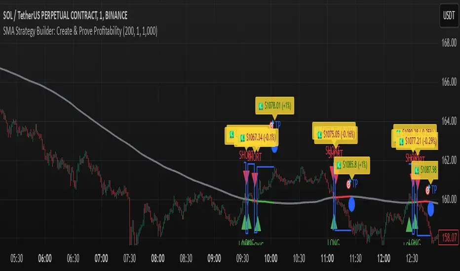
This tool is designed for traders who want to build, customize, and prove their own SMA-based trading strategies. The strategy tracks capital growth in real-time, providing clear evidence of profitability after each trade. Users can adjust key parameters such as SMA period, take profit levels, and initial capital, making it a flexible solution for backtesting and strategy validation.
🔍 Key Features:
✅ SMA-Based Logic:
Core trading logic revolves around the Simple Moving Average (SMA).
SMA period is fully adjustable to suit various trading styles.
🎯 Customizable Take Profit (TP):
User-defined TP percentages per position.
TP line displayed as a Step Line with Breaks for clear segmentation.
Visual 🎯TP label for quick identification of profit targets.
💵 Capital Tracking (Proof of Profitability):
Initial capital is user-defined.
Capital balance updates after each closed trade.
Shows both absolute profit/loss and percentage changes for every position.
Darker green profit labels for better readability and dark red for losses.
📈 Capital Curve (Performance Visualization):
Capital growth curve available (hidden by default, can be enabled via settings).
📏 Dynamic Label Positioning:
Label positions adjust dynamically based on the price range.
Ensures consistent visibility across low and high-priced assets.
⚡ How It Works:
Long Entry:
Triggered when the price crosses above the SMA.
TP level is calculated as a user-defined percentage above the entry price.
Short Entry:
Triggered when the price crosses below the SMA.
TP level is calculated as a user-defined percentage below the entry price.
TP Execution:
Positions close immediately once the TP level is reached (no candle close confirmation needed).
🔔 Alerts:
🟩 Long Signal Alert: When the price crosses above the SMA.
🟥 Short Signal Alert: When the price crosses below the SMA.
🎯 TP Alert: When the TP target is reached.
⚙️ Customization Options:
📅 SMA Period: Choose the moving average period that best fits your strategy.
🎯 Take Profit (%): Adjust TP percentages for flexible risk management.
💵 Initial Capital: Set the starting capital for realistic backtesting.
📈 Capital Curve Toggle: Enable or disable the capital curve to track overall performance.
🌟 Why Use This Tool?
🔧 Flexible Strategy Creation: Adjust core parameters and create tailored SMA-based strategies.
📈 Performance Proof: Capital tracking acts as real proof of profitability after each trade.
🎯 Immediate TP Execution: No waiting for candle closures; profits lock in as soon as targets are hit.
💹 Comprehensive Performance Insights: Percentage-based and absolute capital tracking with dynamic visualization.
🏦 Clean Visual Indicators: Strategy insights made clear with dynamic labeling and adjustable visuals.
⚠️ Disclaimer:
This script is provided for educational and informational purposes only. Trading financial instruments carries risk, and past performance does not guarantee future results. Always perform your own due diligence before making any trading decisions.
Aggressive Strategy for High IV Market### Strategic background
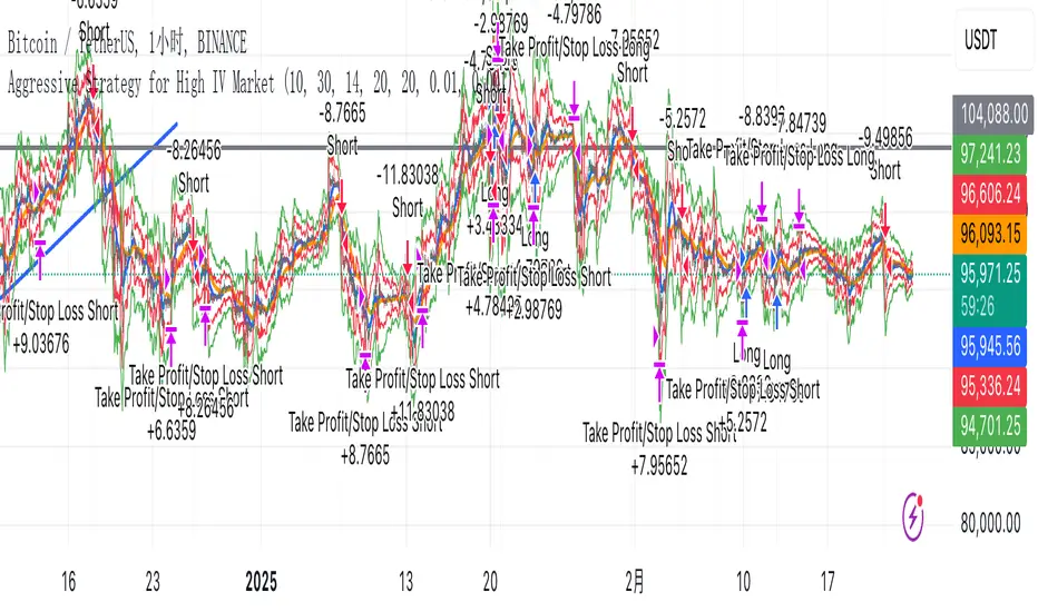
In a volatile high IV market, prices are volatile and market expectations of future uncertainty are high. This environment provides opportunities for aggressive trading strategies, but also comes with a high level of risk. In pursuit of a high Sharpe ratio (i.e., risk-adjusted return), we need to design a strategy that captures the benefits of market volatility while effectively controlling risk. Based on daily line cycles, I choose a combination of trend tracking and volatility filtering for highly volatile assets such as stocks, futures or cryptocurrencies.
---
### Strategy framework
#### Data
- Use daily data, including opening, closing, high and low prices.
- Suitable for highly volatile markets such as technology stocks, cryptocurrencies or volatile index futures.
#### Core indicators
1. ** Trend Indicators ** :
Fast Exponential Moving Average (EMA_fast) : 10-day EMA, used to capture short-term trends.
- Slow Exponential Moving Average (EMA_slow) : 30-day EMA, used to determine the long-term trend.
2. ** Volatility Indicators ** :
Average true Volatility (ATR) : 14-day ATR, used to measure market volatility.
- ATR mean (ATR_mean) : A simple moving average of the 20-day ATR that serves as a volatility benchmark.
- ATR standard deviation (ATR_std) : The standard deviation of the 20-day ATR, which is used to judge extreme changes in volatility.
#### Trading logic
The strategy is based on a trend following approach of double moving averages and filters volatility through ATR indicators, ensuring that trading only in a high-volatility environment is in line with aggressive and high sharpe ratio goals.
---
### Entry and exit conditions
#### Admission conditions
- ** Multiple entry ** :
- EMA_fast Crosses EMA_slow (gold cross), indicating that the short-term trend is turning upward.
-ATR > ATR_mean + 1 * ATR_std indicates that the current volatility is above average and the market is in a state of high volatility.
- ** Short Entry ** :
- EMA_fast Crosses EMA_slow (dead cross) downward, indicating that the short-term trend turns downward.
-ATR > ATR_mean + 1 * ATR_std, confirming high volatility.
#### Appearance conditions
- ** Long show ** :
- EMA_fast Enters the EMA_slow (dead cross) downward, and the trend reverses.
- or ATR < ATR_mean-1 * ATR_std, volatility decreases significantly and the market calms down.
- ** Bear out ** :
- EMA_fast Crosses the EMA_slow (gold cross) on the top, and the trend reverses.
- or ATR < ATR_mean-1 * ATR_std, the volatility is reduced.
---
### Risk management
To control the high risk associated with aggressive strategies, set up the following mechanisms:
1. ** Stop loss ** :
- Long: Entry price - 2 * ATR.
- Short: Entry price + 2 * ATR.
- Dynamic stop loss based on ATR can adapt to market volatility changes.
2. ** Stop profit ** :
- Fixed profit target can be selected (e.g. entry price ± 4 * ATR).
- Or use trailing stop losses to lock in profits following price movements.
3. ** Location Management ** :
- Reduce positions appropriately in times of high volatility, such as dynamically adjusting position size according to ATR, ensuring that the risk of a single trade does not exceed 1%-2% of the account capital.
---
### Strategy features
- ** Aggressiveness ** : By trading only in a high ATR environment, the strategy takes full advantage of market volatility and pursues greater returns.
- ** High Sharpe ratio potential ** : Trend tracking combined with volatility filtering to avoid ineffective trades during periods of low volatility and improve the ratio of return to risk.
- ** Daily line Cycle ** : Based on daily line data, suitable for traders who operate frequently but are not too complex.
---
### Implementation steps
1. ** Data Preparation ** :
- Get the daily data of the target asset.
- Calculate EMA_fast (10 days), EMA_slow (30 days), ATR (14 days), ATR_mean (20 days), and ATR_std (20 days).
2. ** Signal generation ** :
- Check EMA cross signals and ATR conditions daily to generate long/short signals.
3. ** Execute trades ** :
- Enter according to the signal, set stop loss and profit.
- Monitor exit conditions and close positions in time.
4. ** Backtest and Optimization ** :
- Use historical data to backtest strategies to evaluate Sharpe ratios, maximum retracements, and win rates.
- Optimize parameters such as EMA period and ATR threshold to improve policy performance.
---
### Precautions
- ** Trading costs ** : Highly volatile markets may result in frequent trading, and the impact of fees and slippage on earnings needs to be considered.
- ** Risk Control ** : Aggressive strategies may face large retracements and need to strictly implement stop losses.
- ** Scalability ** : Additional metrics (such as volume or VIX) can be added to enhance strategy robustness, or combined with machine learning to predict trends and volatility.
---
### Summary
This is a trend following strategy based on dual moving averages and ATR, designed for volatile high IV markets. By entering into high volatility and exiting into low volatility, the strategy combines aggressive and risk-adjusted returns for traders seeking a high sharpe ratio. It is recommended to fully backtest before implementation and adjust the parameters according to the specific market.
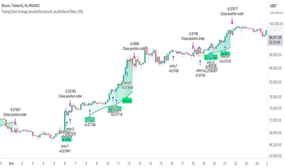
AO/AC Trading Zones Strategy [Skyrexio] Overview
AO/AC Trading Zones Strategy leverages the combination of Awesome Oscillator (AO), Acceleration/Deceleration Indicator (AC), Williams Fractals, Williams Alligator and Exponential Moving Average (EMA) to obtain the high probability long setups. Moreover, strategy uses multi trades system, adding funds to long position if it considered that current trend has likely became stronger. Combination of AO and AC is used for creating so-called trading zones to create the signals, while Alligator and Fractal are used in conjunction as an approximation of short-term trend to filter them. At the same time EMA (default EMA's period = 100) is used as high probability long-term trend filter to open long trades only if it considers current price action as an uptrend. More information in "Methodology" and "Justification of Methodology" paragraphs. The strategy opens only long trades.
Unique Features
No fixed stop-loss and take profit: Instead of fixed stop-loss level strategy utilizes technical condition obtained by Fractals and Alligator to identify when current uptrend is likely to be over. In some special cases strategy uses AO and AC combination to trail profit (more information in "Methodology" and "Justification of Methodology" paragraphs)
Configurable Trading Periods: Users can tailor the strategy to specific market windows, adapting to different market conditions.
Multilayer trades opening system: strategy uses only 10% of capital in every trade and open up to 5 trades at the same time if script consider current trend as strong one.
Short and long term trend trade filters: strategy uses EMA as high probability long-term trend filter and Alligator and Fractal combination as a short-term one.
Methodology
The strategy opens long trade when the following price met the conditions:
1. Price closed above EMA (by default, period = 100). Crossover is not obligatory.
2. Combination of Alligator and Williams Fractals shall consider current trend as an upward (all details in "Justification of Methodology" paragraph)
3. Both AC and AO shall print two consecutive increasing values. At the price candle close which corresponds to this condition algorithm opens the first long trade with 10% of capital.
4. If combination of Alligator and Williams Fractals shall consider current trend has been changed from up to downtrend, all long trades will be closed, no matter how many trades has been opened.
5. If AO and AC both continue printing the rising values strategy opens the long trade on each candle close with 10% of capital while number of opened trades reaches 5.
6. If AO and AC both has printed 5 rising values in a row algorithm close all trades if candle's low below the low of the 5-th candle with rising AO and AC values in a row.
Script also has additional visuals. If second long trade has been opened simultaneously the Alligator's teeth line is plotted with the green color. Also for every trade in a row from 2 to 5 the label "Buy More" is also plotted just below the teeth line. With every next simultaneously opened trade the green color of the space between teeth and price became less transparent.
Strategy settings
In the inputs window user can setup strategy setting:
EMA Length (by default = 100, period of EMA, used for long-term trend filtering EMA calculation).
User can choose the optimal parameters during backtesting on certain price chart.
Justification of Methodology
Let's explore the key concepts of this strategy and understand how they work together. We'll begin with the simplest: the EMA.
The Exponential Moving Average (EMA) is a type of moving average that assigns greater weight to recent price data, making it more responsive to current market changes compared to the Simple Moving Average (SMA). This tool is widely used in technical analysis to identify trends and generate buy or sell signals. The EMA is calculated as follows:
1.Calculate the Smoothing Multiplier:
Multiplier = 2 / (n + 1), Where n is the number of periods.
2. EMA Calculation
EMA = (Current Price) × Multiplier + (Previous EMA) × (1 − Multiplier)
In this strategy, the EMA acts as a long-term trend filter. For instance, long trades are considered only when the price closes above the EMA (default: 100-period). This increases the likelihood of entering trades aligned with the prevailing trend.
Next, let’s discuss the short-term trend filter, which combines the Williams Alligator and Williams Fractals. Williams Alligator
Developed by Bill Williams, the Alligator is a technical indicator that identifies trends and potential market reversals. It consists of three smoothed moving averages:
Jaw (Blue Line): The slowest of the three, based on a 13-period smoothed moving average shifted 8 bars ahead.
Teeth (Red Line): The medium-speed line, derived from an 8-period smoothed moving average shifted 5 bars forward.
Lips (Green Line): The fastest line, calculated using a 5-period smoothed moving average shifted 3 bars forward.
When the lines diverge and align in order, the "Alligator" is "awake," signaling a strong trend. When the lines overlap or intertwine, the "Alligator" is "asleep," indicating a range-bound or sideways market. This indicator helps traders determine when to enter or avoid trades.
Fractals, another tool by Bill Williams, help identify potential reversal points on a price chart. A fractal forms over at least five consecutive bars, with the middle bar showing either:
Up Fractal: Occurs when the middle bar has a higher high than the two preceding and two following bars, suggesting a potential downward reversal.
Down Fractal: Happens when the middle bar shows a lower low than the surrounding two bars, hinting at a possible upward reversal.
Traders often use fractals alongside other indicators to confirm trends or reversals, enhancing decision-making accuracy.
How do these tools work together in this strategy? Let’s consider an example of an uptrend.
When the price breaks above an up fractal, it signals a potential bullish trend. This occurs because the up fractal represents a shift in market behavior, where a temporary high was formed due to selling pressure. If the price revisits this level and breaks through, it suggests the market sentiment has turned bullish.
The breakout must occur above the Alligator’s teeth line to confirm the trend. A breakout below the teeth is considered invalid, and the downtrend might still persist. Conversely, in a downtrend, the same logic applies with down fractals.
In this strategy if the most recent up fractal breakout occurs above the Alligator's teeth and follows the last down fractal breakout below the teeth, the algorithm identifies an uptrend. Long trades can be opened during this phase if a signal aligns. If the price breaks a down fractal below the teeth line during an uptrend, the strategy assumes the uptrend has ended and closes all open long trades.
By combining the EMA as a long-term trend filter with the Alligator and fractals as short-term filters, this approach increases the likelihood of opening profitable trades while staying aligned with market dynamics.
Now let's talk about the trading zones concept and its signals. To understand this we need to briefly introduce what is AO and AC. The Awesome Oscillator (AO), developed by Bill Williams, is a momentum indicator designed to measure market momentum by contrasting recent price movements with a longer-term historical perspective. It helps traders detect potential trend reversals and assess the strength of ongoing trends.
The formula for AO is as follows:
AO = SMA5(Median Price) − SMA34(Median Price)
where:
Median Price = (High + Low) / 2
SMA5 = 5-period Simple Moving Average of the Median Price
SMA 34 = 34-period Simple Moving Average of the Median Price
The Acceleration/Deceleration (AC) Indicator, introduced by Bill Williams, measures the rate of change in market momentum. It highlights shifts in the driving force of price movements and helps traders spot early signs of trend changes. The AC Indicator is particularly useful for identifying whether the current momentum is accelerating or decelerating, which can indicate potential reversals or continuations. For AC calculation we shall use the AO calculated above is the following formula:
AC = AO − SMA5(AO) , where SMA5(AO)is the 5-period Simple Moving Average of the Awesome Oscillator
When the AC is above the zero line and rising, it suggests accelerating upward momentum.
When the AC is below the zero line and falling, it indicates accelerating downward momentum.
When the AC is below zero line and rising it suggests the decelerating the downtrend momentum. When AC is above the zero line and falling, it suggests the decelerating the uptrend momentum.
Now let's discuss the trading zones concept and how it can create the signal. Zones are created by the combination of AO and AC. We can divide three zone types:
Greed zone: when the AO and AC both are rising
Red zone: when the AO and AC both are decreasing
Gray zone: when one of AO or AC is rising, the other is falling
Gray zone is considered as uncertainty. AC and AO are moving in the opposite direction. Strategy skip such price action to decrease the chance to stuck in the losing trade during potential sideways. Red zone is also not interesting for the algorithm because both indicators consider the trend as bearish, but strategy opens only long trades. It is waiting for the green zone to increase the chance to open trade in the direction of the potential uptrend. When we have 2 candles in a row in the green zone script executes a long trade with 10% of capital.
Two green zone candles in a row is considered by algorithm as a bullish trend, but now so strong, that's the reason why trade is going to be closed when the combination of Alligator and Fractals will consider the the trend change from bullish to bearish. If id did not happens, algorithm starts to count the green zone candles in a row. When we have 5 in a row script change the trade closing condition. Such situation is considered is a high probability strong bull market and all trades will be closed if candle's low will be lower than fifth green zone candle's low. This is used to increase probability to secure the profit. If long trades are initiated, the strategy continues utilizing subsequent signals until the total number of trades reaches a maximum of 5. Each trade uses 10% of capital.
Why we use trading zones signals? If currently strategy algorithm considers the high probability of the short-term uptrend with the Alligator and Fractals combination pointed out above and the long-term trend is also suggested by the EMA filter as bullish. Rising AC and AO values in the direction of the most likely main trend signaling that we have the high probability of the fastest bullish phase on the market. The main idea is to take part in such rapid moves and add trades if this move continues its acceleration according to indicators.
Backtest Results
Operating window: Date range of backtests is 2023.01.01 - 2024.12.31. It is chosen to let the strategy to close all opened positions.
Commission and Slippage: Includes a standard Binance commission of 0.1% and accounts for possible slippage over 5 ticks.
Initial capital: 10000 USDT
Percent of capital used in every trade: 10%
Maximum Single Position Loss: -9.49%
Maximum Single Profit: +24.33%
Net Profit: +4374.70 USDT (+43.75%)
Total Trades: 278 (39.57% win rate)
Profit Factor: 2.203
Maximum Accumulated Loss: 668.16 USDT (-5.43%)
Average Profit per Trade: 15.74 USDT (+1.37%)
Average Trade Duration: 60 hours
How to Use
Add the script to favorites for easy access.
Apply to the desired timeframe and chart (optimal performance observed on 4h BTC/USDT).
Configure settings using the dropdown choice list in the built-in menu.
Set up alerts to automate strategy positions through web hook with the text: {{strategy.order.alert_message}}
Disclaimer:
Educational and informational tool reflecting Skyrex commitment to informed trading. Past performance does not guarantee future results. Test strategies in a simulated environment before live implementation
These results are obtained with realistic parameters representing trading conditions observed at major exchanges such as Binance and with realistic trading portfolio usage parameters.
Bollinger Bands Reversal Strategy Analyzer█ OVERVIEW
The Bollinger Bands Reversal Overlay is a versatile trading tool designed to help traders identify potential reversal opportunities using Bollinger Bands. It provides visual signals, performance metrics, and a detailed table to analyze the effectiveness of reversal-based strategies over a user-defined lookback period.
█ KEY FEATURES
Bollinger Bands Calculation
The indicator calculates the standard Bollinger Bands, consisting of:
A middle band (basis) as the Simple Moving Average (SMA) of the closing price.
An upper band as the basis plus a multiple of the standard deviation.
A lower band as the basis minus a multiple of the standard deviation.
Users can customize the length of the Bollinger Bands and the multiplier for the standard deviation.
Reversal Signals
The indicator identifies potential reversal signals based on the interaction between the price and the Bollinger Bands.
Two entry strategies are available:
Revert Cross: Waits for the price to close back above the lower band (for longs) or below the upper band (for shorts) after crossing it.
Cross Threshold: Triggers a signal as soon as the price crosses the lower band (for longs) or the upper band (for shorts).
Trade Direction
Users can select a trade bias:
Long: Focuses on bullish reversal signals.
Short: Focuses on bearish reversal signals.
Performance Metrics
The indicator calculates and displays the performance of trades over a user-defined lookback period ( barLookback ).
Metrics include:
Win Rate: The percentage of trades that were profitable.
Mean Return: The average return across all trades.
Median Return: The median return across all trades.
These metrics are calculated for each bar in the lookback period, providing insights into the strategy's performance over time.
Visual Signals
The indicator plots buy and sell signals on the chart:
Buy Signals: Displayed as green triangles below the price bars.
Sell Signals: Displayed as red triangles above the price bars.
Performance Table
A customizable table is displayed on the chart, showing the performance metrics for each bar in the lookback period.
The table includes:
Win Rate: Highlighted with gradient colors (green for high win rates, red for low win rates).
Mean Return: Colored based on profitability (green for positive returns, red for negative returns).
Median Return: Colored similarly to the mean return.
Time Filtering
Users can define a specific time window for the indicator to analyze trades, ensuring that performance metrics are calculated only for the desired period.
Customizable Display
The table's font size can be adjusted to suit the user's preference, with options for "Auto," "Small," "Normal," and "Large."
█ PURPOSE
The Bollinger Bands Reversal Overlay is designed to:
Help traders identify high-probability reversal opportunities using Bollinger Bands.
Provide actionable insights into the performance of reversal-based strategies.
Enable users to backtest and optimize their trading strategies by analyzing historical performance metrics.
█ IDEAL USERS
Swing Traders: Looking for reversal opportunities within a trend.
Mean Reversion Traders: Interested in trading price reversals to the mean.
Strategy Developers: Seeking to backtest and refine Bollinger Bands-based strategies.
Performance Analysts: Wanting to evaluate the effectiveness of reversal signals over time.

Bullish Reversal Bar Strategy [Skyrexio]Overview
Bullish Reversal Bar Strategy leverages the combination of candlestick pattern Bullish Reversal Bar (description in Methodology and Justification of Methodology), Williams Alligator indicator and Williams Fractals to create the high probability setups. Candlestick pattern is used for the entering into trade, while the combination of Williams Alligator and Fractals is used for the trend approximation as close condition. Strategy uses only long trades.
Unique Features
No fixed stop-loss and take profit: Instead of fixed stop-loss level strategy utilizes technical condition obtained by Fractals and Alligator or the candlestick pattern invalidation to identify when current uptrend is likely to be over (more information in "Methodology" and "Justification of Methodology" paragraphs)
Configurable Trading Periods: Users can tailor the strategy to specific market windows, adapting to different market conditions.
Trend Trade Filter: strategy uses Alligator and Fractal combination as high probability trend filter.
Methodology
The strategy opens long trade when the following price met the conditions:
1.Current candle's high shall be below the Williams Alligator's lines (Jaw, Lips, Teeth)(all details in "Justification of Methodology" paragraph)
2.Price shall create the candlestick pattern "Bullish Reversal Bar". Optionally if MFI and AO filters are enabled current candle shall have the decreasing AO and at least one of three recent bars shall have the squat state on the MFI (all details in "Justification of Methodology" paragraph)
3.If price breaks through the high of the candle marked as the "Bullish Reversal Bar" the long trade is open at the price one tick above the candle's high
4.Initial stop loss is placed at the Bullish Reversal Bar's candle's low
5.If price hit the Bullish Reversal Bar's low before hitting the entry price potential trade is cancelled
6.If trade is active and initial stop loss has not been hit, trade is closed when the combination of Alligator and Williams Fractals shall consider current trend change from upward to downward.
Strategy settings
In the inputs window user can setup strategy setting:
Enable MFI (if true trades are filtered using Market Facilitation Index (MFI) condition all details in "Justification of Methodology" paragraph), by default = false)
Enable AO (if true trades are filtered using Awesome Oscillator (AO) condition all details in "Justification of Methodology" paragraph), by default = false)
Justification of Methodology
Let's explore the key concepts of this strategy and understand how they work together. The first and key concept is the Bullish Reversal Bar candlestick pattern. This is just the single bar pattern. The rules are simple:
Candle shall be closed in it's upper half
High of this candle shall be below all three Alligator's lines (Jaw, Lips, Teeth)
Next, let’s discuss the short-term trend filter, which combines the Williams Alligator and Williams Fractals. Williams Alligator
Developed by Bill Williams, the Alligator is a technical indicator that identifies trends and potential market reversals. It consists of three smoothed moving averages:
Jaw (Blue Line): The slowest of the three, based on a 13-period smoothed moving average shifted 8 bars ahead.
Teeth (Red Line): The medium-speed line, derived from an 8-period smoothed moving average shifted 5 bars forward.
Lips (Green Line): The fastest line, calculated using a 5-period smoothed moving average shifted 3 bars forward.
When the lines diverge and align in order, the "Alligator" is "awake," signaling a strong trend. When the lines overlap or intertwine, the "Alligator" is "asleep," indicating a range-bound or sideways market. This indicator helps traders determine when to enter or avoid trades.
Fractals, another tool by Bill Williams, help identify potential reversal points on a price chart. A fractal forms over at least five consecutive bars, with the middle bar showing either:
Up Fractal: Occurs when the middle bar has a higher high than the two preceding and two following bars, suggesting a potential downward reversal.
Down Fractal: Happens when the middle bar shows a lower low than the surrounding two bars, hinting at a possible upward reversal.
Traders often use fractals alongside other indicators to confirm trends or reversals, enhancing decision-making accuracy.
How do these tools work together in this strategy? Let’s consider an example of an uptrend.
When the price breaks above an up fractal, it signals a potential bullish trend. This occurs because the up fractal represents a shift in market behavior, where a temporary high was formed due to selling pressure. If the price revisits this level and breaks through, it suggests the market sentiment has turned bullish.
The breakout must occur above the Alligator’s teeth line to confirm the trend. A breakout below the teeth is considered invalid, and the downtrend might still persist. Conversely, in a downtrend, the same logic applies with down fractals.
How we can use all these indicators in this strategy? This strategy is a counter trend one. Candle's high shall be below all Alligator's lines. During this market stage the bullish reversal bar candlestick pattern shall be printed. This bar during the downtrend is a high probability setup for the potential reversal to the upside: bulls were able to close the price in the upper half of a candle. The breaking of its high is a high probability signal that trend change is confirmed and script opens long trade. If market continues going down and break down the bullish reversal bar's low potential trend change has been invalidated and strategy close long trade.
If market really reversed and started moving to the upside strategy waits for the trend change form the downtrend to the uptrend according to approximation of Alligator and Fractals combination. If this change happens strategy close the trade. This approach helps to stay in the long trade while the uptrend continuation is likely and close it if there is a high probability of the uptrend finish.
Optionally users can enable MFI and AO filters. First of all, let's briefly explain what are these two indicators. The Awesome Oscillator (AO), created by Bill Williams, is a momentum-based indicator that evaluates market momentum by comparing recent price activity to a broader historical context. It assists traders in identifying potential trend reversals and gauging trend strength.
AO = SMA5(Median Price) − SMA34(Median Price)
where:
Median Price = (High + Low) / 2
SMA5 = 5-period Simple Moving Average of the Median Price
SMA 34 = 34-period Simple Moving Average of the Median Price
This indicator is filtering signals in the following way: if current AO bar is decreasing this candle can be interpreted as a bullish reversal bar. This logic is applicable because initially this strategy is a trend reversal, it is searching for the high probability setup against the current trend. Decreasing AO is the additional high probability filter of a downtrend.
Let's briefly look what is MFI. The Market Facilitation Index (MFI) is a technical indicator that measures the price movement per unit of volume, helping traders gauge the efficiency of price movement in relation to trading volume. Here's how you can calculate it:
MFI = (High−Low)/Volume
MFI can be used in combination with volume, so we can divide 4 states. Bill Williams introduced these to help traders interpret the interaction between volume and price movement. Here’s a quick summary:
Green Window (Increased MFI & Increased Volume): Indicates strong momentum with both price and volume increasing. Often a sign of trend continuation, as both buying and selling interest are rising.
Fake Window (Increased MFI & Decreased Volume): Shows that price is moving but with lower volume, suggesting weak support for the trend. This can signal a potential end of the current trend.
Squat Window (Decreased MFI & Increased Volume): Shows high volume but little price movement, indicating a tug-of-war between buyers and sellers. This often precedes a breakout as the pressure builds.
Fade Window (Decreased MFI & Decreased Volume): Indicates a lack of interest from both buyers and sellers, leading to lower momentum. This typically happens in range-bound markets and may signal consolidation before a new move.
For our purposes we are interested in squat bars. This is the sign that volume cannot move the price easily. This type of bar increases the probability of trend reversal. In this indicator we added to enable the MFI filter of reversal bars. If potential reversal bar or two preceding bars have squat state this bar can be interpret as a reversal one.
Backtest Results
Operating window: Date range of backtests is 2023.01.01 - 2024.12.31. It is chosen to let the strategy to close all opened positions.
Commission and Slippage: Includes a standard Binance commission of 0.1% and accounts for possible slippage over 5 ticks.
Initial capital: 10000 USDT
Percent of capital used in every trade: 50%
Maximum Single Position Loss: -5.29%
Maximum Single Profit: +29.99%
Net Profit: +5472.66 USDT (+54.73%)
Total Trades: 103 (33.98% win rate)
Profit Factor: 1.634
Maximum Accumulated Loss: 1231.15 USDT (-8.32%)
Average Profit per Trade: 53.13 USDT (+0.94%)
Average Trade Duration: 76 hours
How to Use
Add the script to favorites for easy access.
Apply to the desired timeframe and chart (optimal performance observed on 4h ETH/USDT).
Configure settings using the dropdown choice list in the built-in menu.
Set up alerts to automate strategy positions through web hook with the text: {{strategy.order.alert_message}}
Disclaimer:
Educational and informational tool reflecting Skyrex commitment to informed trading. Past performance does not guarantee future results. Test strategies in a simulated environment before live implementation
These results are obtained with realistic parameters representing trading conditions observed at major exchanges such as Binance and with realistic trading portfolio usage parameters.

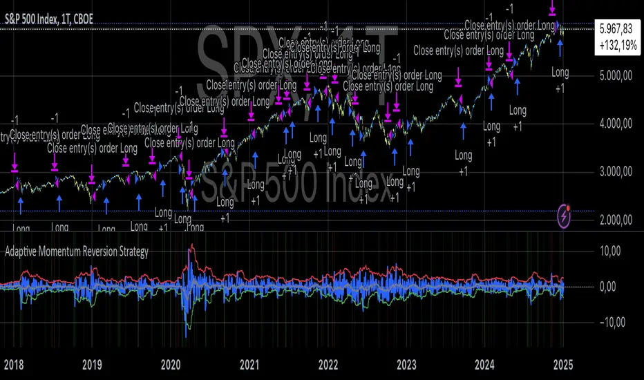
Adaptive Momentum Reversion StrategyThe Adaptive Momentum Reversion Strategy: An Empirical Approach to Market Behavior
The Adaptive Momentum Reversion Strategy seeks to capitalize on market price dynamics by combining concepts from momentum and mean reversion theories. This hybrid approach leverages a Rate of Change (ROC) indicator along with Bollinger Bands to identify overbought and oversold conditions, triggering trades based on the crossing of specific thresholds. The strategy aims to detect momentum shifts and exploit price reversions to their mean.
Theoretical Framework
Momentum and Mean Reversion: Momentum trading assumes that assets with a recent history of strong performance will continue in that direction, while mean reversion suggests that assets tend to return to their historical average over time (Fama & French, 1988; Poterba & Summers, 1988). This strategy incorporates elements of both, looking for periods when momentum is either overextended (and likely to revert) or when the asset’s price is temporarily underpriced relative to its historical trend.
Rate of Change (ROC): The ROC is a straightforward momentum indicator that measures the percentage change in price over a specified period (Wilder, 1978). The strategy calculates the ROC over a 2-period window, making it responsive to short-term price changes. By using ROC, the strategy aims to detect price acceleration and deceleration.
Bollinger Bands: Bollinger Bands are used to identify volatility and potential price extremes, often signaling overbought or oversold conditions. The bands consist of a moving average and two standard deviation bounds that adjust dynamically with price volatility (Bollinger, 2002).
The strategy employs two sets of Bollinger Bands: one for short-term volatility (lower band) and another for longer-term trends (upper band), with different lengths and standard deviation multipliers.
Strategy Construction
Indicator Inputs:
ROC Period: The rate of change is computed over a 2-period window, which provides sensitivity to short-term price fluctuations.
Bollinger Bands:
Lower Band: Calculated with a 18-period length and a standard deviation of 1.7.
Upper Band: Calculated with a 21-period length and a standard deviation of 2.1.
Calculations:
ROC Calculation: The ROC is computed by comparing the current close price to the close price from rocPeriod days ago, expressing it as a percentage.
Bollinger Bands: The strategy calculates both upper and lower Bollinger Bands around the ROC, using a simple moving average as the central basis. The lower Bollinger Band is used as a reference for identifying potential long entry points when the ROC crosses above it, while the upper Bollinger Band serves as a reference for exits, when the ROC crosses below it.
Trading Conditions:
Long Entry: A long position is initiated when the ROC crosses above the lower Bollinger Band, signaling a potential shift from a period of low momentum to an increase in price movement.
Exit Condition: A position is closed when the ROC crosses under the upper Bollinger Band, or when the ROC drops below the lower band again, indicating a reversal or weakening of momentum.
Visual Indicators:
ROC Plot: The ROC is plotted as a line to visualize the momentum direction.
Bollinger Bands: The upper and lower bands, along with their basis (simple moving averages), are plotted to delineate the expected range for the ROC.
Background Color: To enhance decision-making, the strategy colors the background when extreme conditions are detected—green for oversold (ROC below the lower band) and red for overbought (ROC above the upper band), indicating potential reversal zones.
Strategy Performance Considerations
The use of Bollinger Bands in this strategy provides an adaptive framework that adjusts to changing market volatility. When volatility increases, the bands widen, allowing for larger price movements, while during quieter periods, the bands contract, reducing trade signals. This adaptiveness is critical in maintaining strategy effectiveness across different market conditions.
The strategy’s pyramiding setting is disabled (pyramiding=0), ensuring that only one position is taken at a time, which is a conservative risk management approach. Additionally, the strategy includes transaction costs and slippage parameters to account for real-world trading conditions.
Empirical Evidence and Relevance
The combination of momentum and mean reversion has been widely studied and shown to provide profitable opportunities under certain market conditions. Studies such as Jegadeesh and Titman (1993) confirm that momentum strategies tend to work well in trending markets, while mean reversion strategies have been effective during periods of high volatility or after sharp price movements (De Bondt & Thaler, 1985). By integrating both strategies into one system, the Adaptive Momentum Reversion Strategy may be able to capitalize on both trending and reverting market behavior.
Furthermore, research by Chan (1996) on momentum-based trading systems demonstrates that adaptive strategies, which adjust to changes in market volatility, often outperform static strategies, providing a compelling rationale for the use of Bollinger Bands in this context.
Conclusion
The Adaptive Momentum Reversion Strategy provides a robust framework for trading based on the dual concepts of momentum and mean reversion. By using ROC in combination with Bollinger Bands, the strategy is capable of identifying overbought and oversold conditions while adapting to changing market conditions. The use of adaptive indicators ensures that the strategy remains flexible and can perform across different market environments, potentially offering a competitive edge for traders who seek to balance risk and reward in their trading approaches.
References
Bollinger, J. (2002). Bollinger on Bollinger Bands. McGraw-Hill Professional.
Chan, L. K. C. (1996). Momentum, Mean Reversion, and the Cross-Section of Stock Returns. Journal of Finance, 51(5), 1681-1713.
De Bondt, W. F., & Thaler, R. H. (1985). Does the Stock Market Overreact? Journal of Finance, 40(3), 793-805.
Fama, E. F., & French, K. R. (1988). Permanent and Temporary Components of Stock Prices. Journal of Political Economy, 96(2), 246-273.
Jegadeesh, N., & Titman, S. (1993). Returns to Buying Winners and Selling Losers: Implications for Stock Market Efficiency. Journal of Finance, 48(1), 65-91.
Poterba, J. M., & Summers, L. H. (1988). Mean Reversion in Stock Prices: Evidence and Implications. Journal of Financial Economics, 22(1), 27-59.
Wilder, J. W. (1978). New Concepts in Technical Trading Systems. Trend Research.
three Supertrend EMA Strategy by Prasanna +DhanuThe indicator described in your Pine Script is a Supertrend EMA Strategy that combines the Supertrend and EMA (Exponential Moving Average) to create a trend-following strategy. Here’s a detailed breakdown of how this indicator works:
1. EMA (Exponential Moving Average):
The EMA is a moving average that places more weight on recent prices, making it more responsive to price changes compared to a simple moving average (SMA). In this strategy, the EMA is used to determine the overall trend direction.
Input Parameter:
ema_length: This is the period for the EMA, set to 50 periods by default. A shorter EMA will respond more quickly to price movements, while a longer EMA is smoother and less sensitive to short-term fluctuations.
How it's used:
If the price is above the EMA, it indicates an uptrend.
If the price is below the EMA, it indicates a downtrend.
2. Supertrend Indicator:
The Supertrend indicator is a trend-following tool based on the Average True Range (ATR), which is a volatility measure. It helps to identify the direction of the trend by setting a dynamic support or resistance level.
Input Parameters:
supertrend_atr_period: The period used for calculating the ATR, set to 10 periods by default.
supertrend_multiplier1: Multiplier for the first Supertrend, set to 3.0.
supertrend_multiplier2: Multiplier for the second Supertrend, set to 2.0.
supertrend_multiplier3: Multiplier for the third Supertrend, set to 1.0.
Each Supertrend line has a different multiplier, which affects its sensitivity to price changes. The ATR period defines how many periods of price data are used to calculate the ATR.
How the Supertrend works:
If the Supertrend value is below the price, the trend is considered bullish (uptrend).
If the Supertrend value is above the price, the trend is considered bearish (downtrend).
The Supertrend will switch between up and down based on price movement and ATR, providing a dynamic trend-following signal.
3. Three Supertrend Lines:
In this strategy, three Supertrend lines are calculated with different multipliers and the same ATR period (10 periods). Each line is more or less sensitive to price changes, and they are plotted on the chart in different colors based on whether the trend is bullish (green) or bearish (red).
Supertrend 1: The most sensitive Supertrend with a multiplier of 3.0.
Supertrend 2: A moderately sensitive Supertrend with a multiplier of 2.0.
Supertrend 3: The least sensitive Supertrend with a multiplier of 1.0.
Each Supertrend line signals a bullish trend when its value is below the price and a bearish trend when its value is above the price.
4. Strategy Rules:
This strategy uses the three Supertrend lines combined with the EMA to generate trade signals.
Entry Conditions:
A long entry is triggered when all three Supertrend lines are in an uptrend (i.e., all three Supertrend lines are below the price), and the price is above the EMA. This suggests a strong bullish market condition.
A short entry is triggered when all three Supertrend lines are in a downtrend (i.e., all three Supertrend lines are above the price), and the price is below the EMA. This suggests a strong bearish market condition.
Exit Conditions:
A long exit occurs when the third Supertrend (the least sensitive one) switches to a downtrend (i.e., the price falls below it).
A short exit occurs when the third Supertrend switches to an uptrend (i.e., the price rises above it).
5. Visualization:
The strategy also plots the following on the chart:
The EMA is plotted as a blue line, which helps identify the overall trend.
The three Supertrend lines are plotted with different colors:
Supertrend 1: Green (for uptrend) and Red (for downtrend).
Supertrend 2: Green (for uptrend) and Red (for downtrend).
Supertrend 3: Green (for uptrend) and Red (for downtrend).
Summary of the Strategy:
The strategy combines three Supertrend indicators (with different multipliers) and an EMA to capture both short-term and long-term trends.
Long positions are entered when all three Supertrend lines are bullish and the price is above the EMA.
Short positions are entered when all three Supertrend lines are bearish and the price is below the EMA.
Exits occur when the third Supertrend line (the least sensitive) signals a change in trend direction.
This combination of indicators allows for a robust trend-following strategy that adapts to both short-term volatility and long-term trend direction. The Supertrend lines provide quick reaction to price changes, while the EMA offers a smoother, more stable trend direction for confirmation.
The indicator described in your Pine Script is a Supertrend EMA Strategy that combines the Supertrend and EMA (Exponential Moving Average) to create a trend-following strategy. Here’s a detailed breakdown of how this indicator works:
1. EMA (Exponential Moving Average):
The EMA is a moving average that places more weight on recent prices, making it more responsive to price changes compared to a simple moving average (SMA). In this strategy, the EMA is used to determine the overall trend direction.
Input Parameter:
ema_length: This is the period for the EMA, set to 50 periods by default. A shorter EMA will respond more quickly to price movements, while a longer EMA is smoother and less sensitive to short-term fluctuations.
How it's used:
If the price is above the EMA, it indicates an uptrend.
If the price is below the EMA, it indicates a downtrend.
2. Supertrend Indicator:
The Supertrend indicator is a trend-following tool based on the Average True Range (ATR), which is a volatility measure. It helps to identify the direction of the trend by setting a dynamic support or resistance level.
Input Parameters:
supertrend_atr_period: The period used for calculating the ATR, set to 10 periods by default.
supertrend_multiplier1: Multiplier for the first Supertrend, set to 3.0.
supertrend_multiplier2: Multiplier for the second Supertrend, set to 2.0.
supertrend_multiplier3: Multiplier for the third Supertrend, set to 1.0.
Each Supertrend line has a different multiplier, which affects its sensitivity to price changes. The ATR period defines how many periods of price data are used to calculate the ATR.
How the Supertrend works:
If the Supertrend value is below the price, the trend is considered bullish (uptrend).
If the Supertrend value is above the price, the trend is considered bearish (downtrend).
The Supertrend will switch between up and down based on price movement and ATR, providing a dynamic trend-following signal.
3. Three Supertrend Lines:
In this strategy, three Supertrend lines are calculated with different multipliers and the same ATR period (10 periods). Each line is more or less sensitive to price changes, and they are plotted on the chart in different colors based on whether the trend is bullish (green) or bearish (red).
Supertrend 1: The most sensitive Supertrend with a multiplier of 3.0.
Supertrend 2: A moderately sensitive Supertrend with a multiplier of 2.0.
Supertrend 3: The least sensitive Supertrend with a multiplier of 1.0.
Each Supertrend line signals a bullish trend when its value is below the price and a bearish trend when its value is above the price.
4. Strategy Rules:
This strategy uses the three Supertrend lines combined with the EMA to generate trade signals.
Entry Conditions:
A long entry is triggered when all three Supertrend lines are in an uptrend (i.e., all three Supertrend lines are below the price), and the price is above the EMA. This suggests a strong bullish market condition.
A short entry is triggered when all three Supertrend lines are in a downtrend (i.e., all three Supertrend lines are above the price), and the price is below the EMA. This suggests a strong bearish market condition.
Exit Conditions:
A long exit occurs when the third Supertrend (the least sensitive one) switches to a downtrend (i.e., the price falls below it).
A short exit occurs when the third Supertrend switches to an uptrend (i.e., the price rises above it).
5. Visualization:
The strategy also plots the following on the chart:
The EMA is plotted as a blue line, which helps identify the overall trend.
The three Supertrend lines are plotted with different colors:
Supertrend 1: Green (for uptrend) and Red (for downtrend).
Supertrend 2: Green (for uptrend) and Red (for downtrend).
Supertrend 3: Green (for uptrend) and Red (for downtrend).
Summary of the Strategy:
The strategy combines three Supertrend indicators (with different multipliers) and an EMA to capture both short-term and long-term trends.
Long positions are entered when all three Supertrend lines are bullish and the price is above the EMA.
Short positions are entered when all three Supertrend lines are bearish and the price is below the EMA.
Exits occur when the third Supertrend line (the least sensitive) signals a change in trend direction.
This combination of indicators allows for a robust trend-following strategy that adapts to both short-term volatility and long-term trend direction. The Supertrend lines provide quick reaction to price changes, while the EMA offers a smoother, more stable trend direction for confirmation.

Custom Strategy: ETH Martingale 2.0Strategic characteristics
ETH Little Martin 2.0 is a self-developed trading strategy based on the Martingale strategy, mainly used for trading ETH (Ethereum). The core idea of this strategy is to place orders in the same direction at a fixed price interval, and then use Martin's multiple investment principle to reduce losses, but this is also the main source of losses.
Parameter description:
1 Interval: The minimum spacing for taking profit, stop loss, and opening/closing of orders. Different targets have different spacing. Taking ETH as an example, it is generally recommended to have a spacing of 2% for fluctuations in the target.
2 Base Price: This is the price at which you triggered the first order. Similarly, I am using ETH as an example. If you have other targets, I suggest using the initial value of a price that can be backtesting. The Base Price is only an initial order price and has no impact on subsequent orders.
3 Initial Order Amount: Users can set an initial order amount to control the risk of each transaction. If the stop loss is reached, we will double the amount based on this value. This refers to the value of the position held, not the number of positions held.
4 Loss Multiplier: The strategy will increase the next order amount based on the set multiple after the stop loss, in order to make up for the previous losses through a larger position. Note that after taking profit, it will be reset to 1 times the Initial Order Amount.
5. Long Short Operation: The first order of the strategy is a multiple entry, and in subsequent orders, if the stop loss is reached, a reverse order will be opened. The position value of a one-way order is based on the Loss Multiplier multiple investment, so it is generally recommended that the Loss Multiplier default to 2.
Improvement direction
Although this strategy already has a certain trading logic, there are still some improvement directions that can be considered:
1. Dynamic adjustment of spacing: Currently, the spacing is fixed, and it can be considered to dynamically adjust the spacing based on market volatility to improve the adaptability of the strategy. Try using dynamic spacing, which may be more suitable for the actual market situation.
2. Filtering criteria: Orders and no orders can be optimized separately. The biggest problem with this strategy is that it will result in continuous losses during fluctuations, and eventually increase the investment amount. You can consider filtering out some fluctuations or only focusing on trend trends.
3. Risk management: Add more risk management measures, such as setting a maximum loss limit to avoid huge losses caused by continuous stop loss.
4. Optimize the stop loss multiple: Currently, the stop loss multiple is fixed, and it can be considered to dynamically adjust the multiple according to market conditions to reduce risk.

Bollinger Breakout Strategy with Direction Control [4H crypto]Bollinger Breakout Strategy with Direction Control - User Guide
This strategy leverages Bollinger Bands, RSI, and directional filters to identify potential breakout trading opportunities. It is designed for traders looking to capitalize on significant price movements while maintaining control over trade direction (long, short, or both). Here’s how to use this strategy effectively:
How the Strategy Works
Indicators Used:
Bollinger Bands:
A volatility-based indicator with an upper and lower band around a simple moving average (SMA). The bands expand or contract based on market volatility.
RSI (Relative Strength Index):
Measures momentum to determine overbought or oversold conditions. In this strategy, RSI is used to confirm breakout strength.
Trade Direction Control:
You can select whether to trade:
Long only: Buy positions.
Short only: Sell positions.
Both: Trade in both directions depending on conditions.
Breakout Conditions:
Long Trade:
The price closes above the upper Bollinger Band.
RSI is above the midline (50), confirming upward momentum.
The "Trade Direction" setting allows either "Long" or "Both."
Short Trade:
The price closes below the lower Bollinger Band.
RSI is below the midline (50), confirming downward momentum.
The "Trade Direction" setting allows either "Short" or "Both."
Risk Management:
Stop-Loss:
Long trades: Set at 2% below the entry price.
Short trades: Set at 2% above the entry price.
Take-Profit:
Calculated using a Risk/Reward Ratio (default is 2:1).
Adjust this in the strategy settings.
Inputs and Customization
Key Parameters:
Bollinger Bands Length: Default is 20. Adjust based on the desired sensitivity.
Multiplier: Default is 2.0. Higher values widen the bands; lower values narrow them.
RSI Length: Default is 14, which is standard for RSI.
Risk/Reward Ratio: Default is 2.0. Increase for more aggressive profit targets, decrease for conservative exits.
Trade Direction:
Options: "Long," "Short," or "Both."
Example: Set to "Long" in a bullish market to focus only on buy trades.
How to Use This Strategy
Adding the Strategy:
Paste the script into TradingView’s Pine Editor and add it to your chart.
Setting Parameters:
Adjust the Bollinger Band settings, RSI, and Risk/Reward Ratio to fit the asset and timeframe you're trading.
Analyzing Signals:
Green line (Upper Band): Signals breakout potential for long trades.
Red line (Lower Band): Signals breakout potential for short trades.
Blue line (Basis): Central Bollinger Band (SMA), helpful for understanding price trends.
Testing the Strategy:
Use the Strategy Tester in TradingView to backtest performance on your chosen asset and timeframe.
Optimizing for Assets:
Forex pairs, cryptocurrencies (like BTC), or stocks with high volatility are ideal for this strategy.
Works best on higher timeframes like 4H or Daily.
Best Practices
Combine with Volume: Confirm breakouts with increased volume for higher reliability.
Avoid Sideways Markets: Use additional trend filters (like ADX) to avoid trades in low-volatility conditions.
Optimize Parameters: Regularly adjust the Bollinger Bands multiplier and RSI settings to match the asset's behavior.
By utilizing this strategy, you can effectively trade breakouts while maintaining flexibility in trade direction. Adjust the parameters to match your trading style and market conditions for optimal results!

Triple CCI Strategy MFI Confirmed [Skyrexio]Overview
Triple CCI Strategy MFI Confirmed leverages 3 different periods Commodity Channel Index (CCI) indicator in conjunction Money Flow Index (MFI) and Exponential Moving Average (EMA) to obtain the high probability setups. Fast period CCI is used for having the high probability to enter in the direction of short term trend, middle and slow period CCI are used for confirmation, if market now likely in the mid and long-term uptrend. MFI is used to confirm trade with the money inflow/outflow with the high probability. EMA is used as an additional trend filter. Moreover, strategy uses exponential moving average (EMA) to trail the price when it reaches the specific level. More information in "Methodology" and "Justification of Methodology" paragraphs. The strategy opens only long trades.
Unique Features
Dynamic stop-loss system: Instead of fixed stop-loss level strategy utilizes average true range (ATR) multiplied by user given number subtracted from the position entry price as a dynamic stop loss level.
Configurable Trading Periods: Users can tailor the strategy to specific market windows, adapting to different market conditions.
Four layers trade filtering system: Strategy utilizes two different period CCI indicators, MFI and EMA indicators to confirm the signals produced by fast period CCI.
Trailing take profit level: After reaching the trailing profit activation level scrip activate the trailing of long trade using EMA. More information in methodology.
Methodology
The strategy opens long trade when the following price met the conditions:
Fast period CCI shall crossover the zero-line.
Slow and Middle period CCI shall be above zero-lines.
Price shall close above the EMA. Crossover is not obligatory
MFI shall be above 50
When long trade is executed, strategy set the stop-loss level at the price ATR multiplied by user-given value below the entry price. This level is recalculated on every next candle close, adjusting to the current market volatility.
At the same time strategy set up the trailing stop validation level. When the price crosses the level equals entry price plus ATR multiplied by user-given value script starts to trail the price with EMA. If price closes below EMA long trade is closed. When the trailing starts, script prints the label “Trailing Activated”.
Strategy settings
In the inputs window user can setup the following strategy settings:
ATR Stop Loss (by default = 1.75)
ATR Trailing Profit Activation Level (by default = 2.25)
CCI Fast Length (by default = 14, used for calculation short term period CCI)
CCI Middle Length (by default = 25, used for calculation short term period CCI)
CCI Slow Length (by default = 50, used for calculation long term period CCI)
MFI Length (by default = 14, used for calculation MFI
EMA Length (by default = 50, period of EMA, used for trend filtering EMA calculation)
Trailing EMA Length (by default = 20)
User can choose the optimal parameters during backtesting on certain price chart.
Justification of Methodology
Before understanding why this particular combination of indicator has been chosen let's briefly explain what is CCI, MFI and EMA.
The Commodity Channel Index (CCI) is a momentum-based technical indicator that measures the deviation of a security's price from its average price over a specific period. It helps traders identify overbought or oversold conditions and potential trend reversals.
The CCI formula is:
CCI = (Typical Price − SMA) / (0.015 × Mean Deviation)
Typical Price (TP): This is calculated as the average of the high, low, and closing prices for the period.
Simple Moving Average (SMA): This is the average of the Typical Prices over a specific number of periods.
Mean Deviation: This is the average of the absolute differences between the Typical Price and the SMA.
The result is a value that typically fluctuates between +100 and -100, though it is not bounded and can go higher or lower depending on the price movement.
The Money Flow Index (MFI) is a technical indicator that measures the strength of money flowing into and out of a security. It combines price and volume data to assess buying and selling pressure and is often used to identify overbought or oversold conditions. The formula for MFI involves several steps:
1. Calculate the Typical Price (TP):
TP = (high + low + close) / 3
2. Calculate the Raw Money Flow (RMF):
Raw Money Flow = TP × Volume
3. Determine Positive and Negative Money Flow:
If the current TP is greater than the previous TP, it's Positive Money Flow.
If the current TP is less than the previous TP, it's Negative Money Flow.
4. Calculate the Money Flow Ratio (MFR):
Money Flow Ratio = Sum of Positive Money Flow (over n periods) / Sum of Negative Money Flow (over n periods)
5. Calculate the Money Flow Index (MFI):
MFI = 100 − (100 / (1 + Money Flow Ratio))
MFI above 80 can be considered as overbought, below 20 - oversold.
The Exponential Moving Average (EMA) is a type of moving average that places greater weight and significance on the most recent data points. It is widely used in technical analysis to smooth price data and identify trends more quickly than the Simple Moving Average (SMA).
Formula:
1. Calculate the multiplier
Multiplier = 2 / (n + 1) , Where n is the number of periods.
2. EMA Calculation
EMA = (Current Price) × Multiplier + (Previous EMA) × (1 − Multiplier)
This strategy leverages Fast period CCI, which shall break the zero line to the upside to say that probability of short term trend change to the upside increased. This zero line crossover shall be confirmed by the Middle and Slow periods CCI Indicators. At the moment of breakout these two CCIs shall be above 0, indicating that there is a high probability that price is in middle and long term uptrend. This approach increases chances to have a long trade setup in the direction of mid-term and long-term trends when the short-term trend starts to reverse to the upside.
Additionally strategy uses MFI to have a greater probability that fast CCI breakout is confirmed by this indicator. We consider the values of MFI above 50 as a higher probability that trend change from downtrend to the uptrend is real. Script opens long trades only if MFI is above 50. As you already know from the MFI description, it incorporates volume in its calculation, therefore we have another one confirmation factor.
Finally, strategy uses EMA an additional trend filter. It allows to open long trades only if price close above EMA (by default 50 period). It increases the probability of taking long trades only in the direction of the trend.
ATR is used to adjust the strategy risk management to the current market volatility. If volatility is low, we don’t need the large stop loss to understand the there is a high probability that we made a mistake opening the trade. User can setup the settings ATR Stop Loss and ATR Trailing Profit Activation Level to realize his own risk to reward preferences, but the unique feature of a strategy is that after reaching trailing profit activation level strategy is trying to follow the trend until it is likely to be finished instead of using fixed risk management settings. It allows sometimes to be involved in the large movements. It’s also important to make a note, that script uses another one EMA (by default = 20 period) as a trailing profit level.
Backtest Results
Operating window: Date range of backtests is 2022.04.01 - 2024.11.25. It is chosen to let the strategy to close all opened positions.
Commission and Slippage: Includes a standard Binance commission of 0.1% and accounts for possible slippage over 5 ticks.
Initial capital: 10000 USDT
Percent of capital used in every trade: 50%
Maximum Single Position Loss: -4.13%
Maximum Single Profit: +19.66%
Net Profit: +5421.21 USDT (+54.21%)
Total Trades: 108 (44.44% win rate)
Profit Factor: 2.006
Maximum Accumulated Loss: 777.40 USDT (-7.77%)
Average Profit per Trade: 50.20 USDT (+0.85%)
Average Trade Duration: 44 hours
These results are obtained with realistic parameters representing trading conditions observed at major exchanges such as Binance and with realistic trading portfolio usage parameters.
How to Use
Add the script to favorites for easy access.
Apply to the desired timeframe and chart (optimal performance observed on 2h BTC/USDT).
Configure settings using the dropdown choice list in the built-in menu.
Set up alerts to automate strategy positions through web hook with the text: {{strategy.order.alert_message}}
Disclaimer:
Educational and informational tool reflecting Skyrex commitment to informed trading. Past performance does not guarantee future results. Test strategies in a simulated environment before live implementation
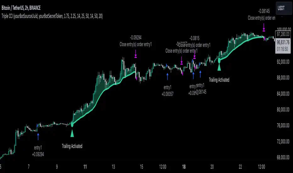
Dual Strategy Selector V2 - CryptogyaniOverview:
This script provides traders with a dual-strategy system that they can toggle between using a simple dropdown menu in the input settings. It is designed to cater to different trading styles and needs, offering both simplicity and advanced filtering techniques. The strategies are built around moving average crossovers, enhanced by configurable risk management tools like take profit levels, trailing stops, and ATR-based stop-loss.
Key Features:
Two Strategies in One Script:
Strategy 1: A classic moving average crossover strategy for identifying entry signals based on trend reversals. Includes user-defined take profit and trailing stop-loss options for profit locking.
Strategy 2: An advanced trend-following system that incorporates:
A higher timeframe trend filter to confirm entry signals.
ATR-based stop-loss for dynamic risk management.
Configurable partial take profit to secure gains while letting the trade run.
Highly Customizable:
All key parameters such as SMA lengths, take profit levels, ATR multiplier, and timeframe for the trend filter are adjustable via the input settings.
Dynamic Toggle:
Traders can switch between Strategy 1 and Strategy 2 with a single dropdown, allowing them to adapt the strategy to market conditions.
How It Works:
Strategy 1:
Entry Logic: A long trade is triggered when the fast SMA crosses above the slow SMA.
Exit Logic: The trade exits at either a user-defined take profit level (percentage or pips) or via an optional trailing stop that dynamically adjusts based on price movement.
Strategy 2:
Entry Logic: Builds on the SMA crossover logic but adds a higher timeframe trend filter to align trades with the broader market direction.
Risk Management:
ATR-Based Stop-Loss: Protects against adverse moves with a volatility-adjusted stop-loss.
Partial Take Profit: Allows traders to secure a percentage of gains while keeping some exposure for extended trends.
How to Use:
Select Your Strategy:
Use the dropdown in the input settings to choose Strategy 1 or Strategy 2.
Configure Parameters:
Adjust SMA lengths, take profit, and risk management settings to align with your trading style.
For Strategy 2, specify the higher timeframe for trend filtering.
Deploy and Monitor:
Apply the script to your preferred asset and timeframe.
Use the backtest results to fine-tune settings for optimal performance.
Why Choose This Script?:
This script stands out due to its dual-strategy flexibility and enhanced features:
For beginners: Strategy 1 provides a simple yet effective trend-following system with minimal setup.
For advanced traders: Strategy 2 includes powerful tools like trend filters and ATR-based stop-loss, making it ideal for challenging market conditions.
By combining simplicity with advanced features, this script offers something for everyone while maintaining full transparency and user customization.
Default Settings:
Strategy 1:
Fast SMA: 21, Slow SMA: 49
Take Profit: 7% or 50 pips
Trailing Stop: Optional (disabled by default)
Strategy 2:
Fast SMA: 20, Slow SMA: 50
ATR Multiplier: 1.5
Partial Take Profit: 50%
Higher Timeframe: 1 Day (1D)
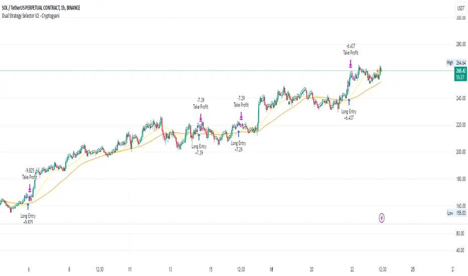
Max Pain StrategyThe Max Pain Strategy uses a combination of volume and price movement thresholds to identify potential "pain zones" in the market. A "pain zone" is considered when the volume exceeds a certain multiple of its average over a defined lookback period, and the price movement exceeds a predefined percentage relative to the price at the beginning of the lookback period.
Here’s how the strategy functions step-by-step:
Inputs:
length: Defines the lookback period used to calculate the moving average of volume and the price change over that period.
volMultiplier: Sets a threshold multiplier for the volume; if the volume exceeds the average volume multiplied by this factor, it triggers the condition for a potential "pain zone."
priceMultiplier: Sets a threshold for the minimum percentage price change that is required for a "pain zone" condition.
Calculations:
averageVolume: The simple moving average (SMA) of volume over the specified lookback period.
priceChange: The absolute difference in price between the current bar's close and the close from the lookback period (length).
Pain Zone Condition:
The condition for entering a position is triggered if both the volume is higher than the average volume by the volMultiplier and the price change exceeds the price at the length-period ago by the priceMultiplier. This is an indication of significant market activity that could result in a price move.
Position Entry:
A long position is entered when the "pain zone" condition is met.
Exit Strategy:
The position is closed after the specified holdPeriods, which defines how many periods the position will be held after being entered.
Visualization:
A small triangle is plotted on the chart where the "pain zone" condition is met.
The background color changes to a semi-transparent red when the "pain zone" is active.
Scientific Explanation of the Components
Volume Analysis and Price Movement: These are two critical factors in trading strategies. Volume often serves as an indicator of market strength (or weakness), and price movement is a direct reflection of market sentiment. Higher volume with significant price movement may suggest that the market is entering a phase of increased volatility or trend formation, which the strategy aims to exploit.
Volume analysis: The study of volume as an indicator of market participation, with increased volume often signaling stronger trends (Murphy, J. J., Technical Analysis of the Financial Markets).
Price movement thresholds: A large price change over a short period may be interpreted as a breakout or a potential reversal point, aligning with volatility and liquidity analysis (Schwager, J. D., Market Wizards).
Repainting Check: This strategy does not involve any repainting because it is based on current and past data, and there is no reference to future values in the decision-making process. However, any strategy that uses lagging indicators or conditions based on historical bars, like close , is inherently a lagging strategy and might not predict real-time price action accurately until after the fact.
Risk Management: The position hold duration is predefined, which adds an element of time-based risk control. This duration ensures that the strategy does not hold a position indefinitely, which could expose it to unnecessary risk.
Potential Issues and Considerations
Repainting:
The strategy does not utilize future data or conditions that depend on future bars, so it does not inherently suffer from repainting issues.
However, since the strategy relies on volume and price change over a set lookback period, the decision to enter or exit a trade is only made after the data for the current bar is complete, meaning the trade decisions are somewhat delayed, which could be seen as a lagging feature rather than a repainting one.
Lagging Nature:
As with many technical analysis-based strategies, this one is based on past data (moving averages, price changes), meaning it reacts to market movements after they have already occurred, rather than predicting future price actions.
Overfitting Risk:
With parameters like the lookback period and multipliers being user-adjustable, there is a risk of overfitting to historical data. Adjusting parameters too much based on past performance can lead to poor out-of-sample results (Gauthier, P., Practical Quantitative Finance).
Conclusion
The Max Pain Strategy is a simple approach to identifying potential market entries based on volume spikes and significant price changes. It avoids repainting by relying solely on historical and current bar data, but it is inherently a lagging strategy that reacts to price and volume patterns after they have occurred. Therefore, the strategy can be effective in trending markets but may struggle in highly volatile, sideways markets.

The Most Powerful TQQQ EMA Crossover Trend Trading StrategyTQQQ EMA Crossover Strategy Indicator
Meta Title: TQQQ EMA Crossover Strategy - Enhance Your Trading with Effective Signals
Meta Description: Discover the TQQQ EMA Crossover Strategy, designed to optimize trading decisions with fast and slow EMA crossovers. Learn how to effectively use this powerful indicator for better trading results.
Key Features
The TQQQ EMA Crossover Strategy is a powerful trading tool that utilizes Exponential Moving Averages (EMAs) to identify potential entry and exit points in the market. Key features of this indicator include:
**Fast and Slow EMAs:** The strategy incorporates two EMAs, allowing traders to capture short-term trends while filtering out market noise.
**Entry and Exit Signals:** Automated signals for entering and exiting trades based on EMA crossovers, enhancing decision-making efficiency.
**Customizable Parameters:** Users can adjust the lengths of the EMAs, as well as take profit and stop loss multipliers, tailoring the strategy to their trading style.
**Visual Indicators:** Clear visual plots of the EMAs and exit points on the chart for easy interpretation.
How It Works
The TQQQ EMA Crossover Strategy operates by calculating two EMAs: a fast EMA (default length of 20) and a slow EMA (default length of 50). The core concept is based on the crossover of these two moving averages:
- When the fast EMA crosses above the slow EMA, it generates a *buy signal*, indicating a potential upward trend.
- Conversely, when the fast EMA crosses below the slow EMA, it produces a *sell signal*, suggesting a potential downward trend.
This method allows traders to capitalize on momentum shifts in the market, providing timely signals for trade execution.
Trading Ideas and Insights
Traders can leverage the TQQQ EMA Crossover Strategy in various market conditions. Here are some insights:
**Scalping Opportunities:** The strategy is particularly effective for scalping in volatile markets, allowing traders to make quick profits on small price movements.
**Swing Trading:** Longer-term traders can use this strategy to identify significant trend reversals and capitalize on larger price swings.
**Risk Management:** By incorporating customizable stop loss and take profit levels, traders can manage their risk effectively while maximizing potential returns.
How Multiple Indicators Work Together
While this strategy primarily relies on EMAs, it can be enhanced by integrating additional indicators such as:
- **Relative Strength Index (RSI):** To confirm overbought or oversold conditions before entering trades.
- **Volume Indicators:** To validate breakout signals, ensuring that price movements are supported by sufficient trading volume.
Combining these indicators provides a more comprehensive view of market dynamics, increasing the reliability of trade signals generated by the EMA crossover.
Unique Aspects
What sets this indicator apart is its simplicity combined with effectiveness. The reliance on EMAs allows for smoother signals compared to traditional moving averages, reducing false signals often associated with choppy price action. Additionally, the ability to customize parameters ensures that traders can adapt the strategy to fit their unique trading styles and risk tolerance.
How to Use
To effectively utilize the TQQQ EMA Crossover Strategy:
1. **Add the Indicator:** Load the script onto your TradingView chart.
2. **Set Parameters:** Adjust the fast and slow EMA lengths according to your trading preferences.
3. **Monitor Signals:** Watch for crossover points; enter trades based on buy/sell signals generated by the indicator.
4. **Implement Risk Management:** Set your stop loss and take profit levels using the provided multipliers.
Regularly review your trading performance and adjust parameters as necessary to optimize results.
Customization
The TQQQ EMA Crossover Strategy allows for extensive customization:
- **EMA Lengths:** Change the default lengths of both fast and slow EMAs to suit different time frames or market conditions.
- **Take Profit/Stop Loss Multipliers:** Adjust these values to align with your risk management strategy. For instance, increasing the take profit multiplier may yield larger gains but could also increase exposure to market fluctuations.
This flexibility makes it suitable for various trading styles, from aggressive scalpers to conservative swing traders.
Conclusion
The TQQQ EMA Crossover Strategy is an effective tool for traders seeking an edge in their trading endeavors. By utilizing fast and slow EMAs, this indicator provides clear entry and exit signals while allowing for customization to fit individual trading strategies. Whether you are a scalper looking for quick profits or a swing trader aiming for larger moves, this indicator offers valuable insights into market trends.
Incorporate it into your TradingView toolkit today and elevate your trading performance!

S&P 100 Option Expiration Week StrategyThe Option Expiration Week Strategy aims to capitalize on increased volatility and trading volume that often occur during the week leading up to the expiration of options on stocks in the S&P 100 index. This period, known as the option expiration week, culminates on the third Friday of each month when stock options typically expire in the U.S. During this week, investors in this strategy take a long position in S&P 100 stocks or an equivalent ETF from the Monday preceding the third Friday, holding until Friday. The strategy capitalizes on potential upward price pressures caused by increased option-related trading activity, rebalancing, and hedging practices.
The phenomenon leveraged by this strategy is well-documented in finance literature. Studies demonstrate that options expiration dates have a significant impact on stock returns, trading volume, and volatility. This effect is driven by various market dynamics, including portfolio rebalancing, delta hedging by option market makers, and the unwinding of positions by institutional investors (Stoll & Whaley, 1987; Ni, Pearson, & Poteshman, 2005). These market activities intensify near option expiration, causing price adjustments that may create short-term profitable opportunities for those aware of these patterns (Roll, Schwartz, & Subrahmanyam, 2009).
The paper by Johnson and So (2013), Returns and Option Activity over the Option-Expiration Week for S&P 100 Stocks, provides empirical evidence supporting this strategy. The study analyzes the impact of option expiration on S&P 100 stocks, showing that these stocks tend to exhibit abnormal returns and increased volume during the expiration week. The authors attribute these patterns to intensified option trading activity, where demand for hedging and arbitrage around options expiration causes temporary price adjustments.
Scientific Explanation
Research has found that option expiration weeks are marked by predictable increases in stock returns and volatility, largely due to the role of options market makers and institutional investors. Option market makers often use delta hedging to manage exposure, which requires frequent buying or selling of the underlying stock to maintain a hedged position. As expiration approaches, their activity can amplify price fluctuations. Additionally, institutional investors often roll over or unwind positions during expiration weeks, creating further demand for underlying stocks (Stoll & Whaley, 1987). This increased demand around expiration week typically leads to temporary stock price increases, offering profitable opportunities for short-term strategies.
Key Research and Bibliography
Johnson, T. C., & So, E. C. (2013). Returns and Option Activity over the Option-Expiration Week for S&P 100 Stocks. Journal of Banking and Finance, 37(11), 4226-4240.
This study specifically examines the S&P 100 stocks and demonstrates that option expiration weeks are associated with abnormal returns and trading volume due to increased activity in the options market.
Stoll, H. R., & Whaley, R. E. (1987). Program Trading and Expiration-Day Effects. Financial Analysts Journal, 43(2), 16-28.
Stoll and Whaley analyze how program trading and portfolio insurance strategies around expiration days impact stock prices, leading to temporary volatility and increased trading volume.
Ni, S. X., Pearson, N. D., & Poteshman, A. M. (2005). Stock Price Clustering on Option Expiration Dates. Journal of Financial Economics, 78(1), 49-87.
This paper investigates how option expiration dates affect stock price clustering and volume, driven by delta hedging and other option-related trading activities.
Roll, R., Schwartz, E., & Subrahmanyam, A. (2009). Options Trading Activity and Firm Valuation. Journal of Financial Markets, 12(3), 519-534.
The authors explore how options trading activity influences firm valuation, finding that higher options volume around expiration dates can lead to temporary price movements in underlying stocks.
Cao, C., & Wei, J. (2010). Option Market Liquidity and Stock Return Volatility. Journal of Financial and Quantitative Analysis, 45(2), 481-507.
This study examines the relationship between options market liquidity and stock return volatility, finding that increased liquidity needs during expiration weeks can heighten volatility, impacting stock returns.
Summary
The Option Expiration Week Strategy utilizes well-researched financial market phenomena related to option expiration. By positioning long in S&P 100 stocks or ETFs during this period, traders can potentially capture abnormal returns driven by option market dynamics. The literature suggests that options-related activities—such as delta hedging, position rollovers, and portfolio adjustments—intensify demand for underlying assets, creating short-term profit opportunities around these key dates.

FS Scorpion TailKey Features & Components:
1. Custom Date & Chart-Based Controls
The software allows users to define whether they want signals to start on a specific date (useSpecificDate) or base calculations on the visible chart’s range (useRelativeScreenSumLeft and useRelativeScreenSumRight).
Users can input the number of stocks to buy/sell per signal and decide whether to sell only for profit.
2. Technical Indicators Used
EMA (Exponential Moving Average): Users can define the length of the EMA and specify if buy/sell signals should occur when the EMA is rising or falling.
MACD (Moving Average Convergence Divergence): MACD crossovers, slopes of the MACD line, signal line, and histogram are used for generating buy/sell signals.
ATR (Average True Range): Signals are generated based on rising or falling ATR.
Aroon Indicator: Buy and sell signals are based on the behavior of the Aroon upper and lower lines.
RSI (Relative Strength Index): Tracks whether the RSI and its moving average are rising or falling to generate signals.
Bollinger Bands: Buy/sell signals depend on the basis, upper, and lower band behavior (rising or falling).
3. Signal Detection
The software creates arrays for each indicator to store conditions for buy/sell signals.
The allTrue() function checks whether all conditions for buy/sell signals are true, ensuring that only valid signals are plotted.
Signals are differentiated between buy-only, sell-only, and both buy and sell (dual signal).
4. Visual Indicators
Vertical Lines: When buy, sell, or dual signals are detected, vertical lines are drawn at the corresponding bar with configurable colors (green for buy, red for sell, silver for dual).
Buy/Sell Labels: Visual labels are plotted directly on the chart to denote buy or sell signals, allowing for clear interpretation of the strategy.
5. Cash Flow & Metrics Display
The software maintains an internal ledger of how many stocks are bought/sold, their prices, and whether a profit is being made.
A table is displayed at the bottom right of the chart, showing:
Initial investment
Current stocks owned
Last buy price
Market stake
Net profit
The table background turns green for profit and red for loss.
6. Dynamic Decision Making
Buy Condition: If a valid buy signal is generated, the software decrements the cash balance and adds stocks to the inventory.
Sell Condition: If the sell signal is valid (and meets the profit requirement), stocks are sold, and cash is incremented.
A fallback check ensures the sell logic prevents selling more stocks than are available and adjusts stock holding appropriately (e.g., sell half).
Customization and Usage
Indicator Adjustments: The user can choose which indicators to activate (e.g., EMA, MACD, RSI) via input controls. Each indicator has specific customizable parameters such as lengths, slopes, and conditions.
Signal Flexibility: The user can adjust conditions for buying and selling based on various technical indicators, which adds flexibility in implementing trading strategies. For example, users may require the RSI to be higher than its moving average or trigger sales only when MACD crosses under the signal line.
Profit Sensitivity: The software allows the option to sell only when a profit is assured by checking if the current price is higher than the last buy price.
Summary of Usage:
Indicator Selection: Enable or disable technical indicators like EMA, MACD, RSI, Aroon, ATR, and Bollinger Bands to fit your trading strategy.
Custom Date/Chart Settings: Choose whether to calculate based on specific time ranges or visible portions of the chart.
Dynamic Signal Plotting: Once buy or sell conditions are met, the software will visually plot signals on your chart, giving clear entry and exit points.
Investment Tracking: Real-time tracking of stock quantities, investments, and profit ensures a clear view of your trading performance.
Backtesting: Use this software for backtesting your strategy by analyzing how buy and sell signals would have performed historically based on the chosen indicators.
Conclusion
The FS Scorpion Tail software is a robust and flexible trading tool, allowing traders to develop custom strategies based on multiple well-known technical indicators. Its visual aid, coupled with real-time investment tracking, makes it valuable for systematic traders looking to automate or refine their trading approach.

Bollinger Bands Mean Reversion by Kevin Davey Bollinger Bands Mean Reversion Strategy Description
The Bollinger Bands Mean Reversion Strategy is a popular trading approach based on the concept of volatility and market overreaction. The strategy leverages Bollinger Bands, which consist of an upper and lower band plotted around a central moving average, typically using standard deviations to measure volatility. When the price moves beyond these bands, it signals potential overbought or oversold conditions, and the strategy seeks to exploit a reversion back to the mean (the central band).
Strategy Components:
1. Bollinger Bands:
The bands are calculated using a 20-period Simple Moving Average (SMA) and a multiple (usually 2.0) of the standard deviation of the asset’s price over the same period. The upper band represents the SMA plus two standard deviations, while the lower band is the SMA minus two standard deviations. The distance between the bands increases with higher volatility and decreases with lower volatility.
2. Mean Reversion:
Mean reversion theory suggests that, over time, prices tend to move back toward their historical average. In this strategy, a buy signal is triggered when the price falls below the lower Bollinger Band, indicating a potential oversold condition. Conversely, the position is closed when the price rises back above the upper Bollinger Band, signaling an overbought condition.
Entry and Exit Logic:
Buy Condition: The strategy enters a long position when the price closes below the lower Bollinger Band, anticipating a mean reversion to the central band (SMA).
Sell Condition: The long position is exited when the price closes above the upper Bollinger Band, implying that the market is likely overbought and a reversal could occur.
This approach uses mean reversion principles, aiming to capitalize on short-term price extremes and volatility compression, often seen in sideways or non-trending markets. Scientific studies have shown that mean reversion strategies, particularly those based on volatility indicators like Bollinger Bands, can be effective in capturing small but frequent price reversals  .
Scientific Basis for Bollinger Bands:
Bollinger Bands, developed by John Bollinger, are widely regarded in both academic literature and practical trading as an essential tool for volatility analysis and mean reversion strategies. Research has shown that Bollinger Bands effectively identify relative price highs and lows, and can be used to forecast price volatility and detect potential breakouts . Studies in financial markets, such as those by Fernández-Rodríguez et al. (2003), highlight the efficacy of Bollinger Bands in detecting overbought or oversold conditions in various assets .
Who is Kevin Davey?
Kevin Davey is an award-winning algorithmic trader and highly regarded expert in developing and optimizing systematic trading strategies. With over 25 years of experience, Davey gained significant recognition after winning the prestigious World Cup Trading Championships multiple times, where he achieved triple-digit returns with minimal drawdown. His success has made him a key figure in algorithmic trading education, with a focus on disciplined and rule-based trading systems.

Unlock the Power of Seasonality: Monthly Performance StrategyThe Monthly Performance Strategy leverages the power of seasonality—those cyclical patterns that emerge in financial markets at specific times of the year. From tax deadlines to industry-specific events and global holidays, historical data shows that certain months can offer strong opportunities for trading. This strategy was designed to help traders capture those opportunities and take advantage of recurring market patterns through an automated and highly customizable approach.
The Inspiration Behind the Strategy:
This strategy began with the idea that market performance is often influenced by seasonal factors. Historically, certain months outperform others due to a variety of reasons, like earnings reports, holiday shopping, or fiscal year-end events. By identifying these periods, traders can better time their market entries and exits, giving them an advantage over those who solely rely on technical indicators or news events.
The Monthly Performance Strategy was built to take this concept and automate it. Instead of manually analyzing market data for each month, this strategy enables you to select which months you want to focus on and then executes trades based on predefined rules, saving you time and optimizing the performance of your trades.
Key Features:
Customizable Month Selection: The strategy allows traders to choose specific months to test or trade on. You can select any combination of months—for example, January, July, and December—to focus on based on historical trends. Whether you’re targeting the historically strong months like December (often driven by the 'Santa Rally') or analyzing quieter months for low volatility trades, this strategy gives you full control.
Automated Monthly Entries and Exits: The strategy automatically enters a long position on the first day of your selected month(s) and exits the trade at the beginning of the next month. This makes it perfect for traders who want to benefit from seasonal patterns without manually monitoring the market. It ensures precision in entering and exiting trades based on pre-set timeframes.
Re-entry on Stop Loss or Take Profit: One of the standout features of this strategy is its ability to re-enter a trade if a position hits the stop loss (SL) or take profit (TP) level during the selected month. If your trade reaches either a SL or TP before the month ends, the strategy will automatically re-enter a new trade the next trading day. This feature ensures that you capture multiple trading opportunities within the same month, instead of exiting entirely after a successful or unsuccessful trade. Essentially, it keeps your capital working for you throughout the entire month, not just when conditions align perfectly at the beginning.
Built-in Risk Management: Risk management is a vital part of this strategy. It incorporates an Average True Range (ATR)-based stop loss and take profit system. The ATR helps set dynamic levels based on the market’s volatility, ensuring that your stops and targets adjust to changing market conditions. This not only helps limit potential losses but also maximizes profit potential by adapting to market behavior.
Historical Performance Testing: You can backtest this strategy on any period by setting the start year. This allows traders to analyze past market data and optimize their strategy based on historical performance. You can fine-tune which months to trade based on years of data, helping you identify trends and patterns that provide the best trading results.
Versatility Across Asset Classes: While this strategy can be particularly effective for stock market indices and sector rotation, it’s versatile enough to apply to other asset classes like forex, commodities, and even cryptocurrencies. Each asset class may exhibit different seasonal behaviors, allowing you to explore opportunities across various markets with this strategy.
How It Works:
The trader selects which months to test or trade, for example, January, April, and October.
The strategy will automatically open a long position on the first trading day of each selected month.
If the trade hits either the take profit or stop loss within the month, the strategy will close the current position and re-enter a new trade on the next trading day, provided the month has not yet ended. This ensures that the strategy continues to capture any potential gains throughout the month, rather than stopping after one successful trade.
At the start of the next month, the position is closed, and if the next month is also selected, a new trade is initiated following the same process.
Risk Management and Dynamic Adjustments:
Incorporating risk management with this strategy is as easy as turning on the ATR-based system. The strategy will automatically calculate stop loss and take profit levels based on the market’s current volatility, adjusting dynamically to the conditions. This ensures that the risk is controlled while allowing for flexibility in capturing profits during both high and low volatility periods.
Maximizing the Seasonal Edge:
By automating entries and exits based on specific months and combining that with dynamic risk management, the Ultimate Monthly Performance Strategy takes advantage of seasonal patterns without requiring constant monitoring. The added re-entry feature after hitting a stop loss or take profit ensures that you are always in the game, maximizing your chances to capture profitable trades during favorable seasonal periods.
Who Can Benefit from This Strategy?
This strategy is perfect for traders who:
Want to exploit the predictable, recurring patterns that occur during specific months of the year.
Prefer a hands-off, automated trading approach that allows them to focus on other aspects of their portfolio or life.
Seek to manage risk effectively with ATR-based stop losses and take profits that adjust to market conditions.
Appreciate the ability to re-enter trades when a take profit or stop loss is hit within the month, ensuring that they don't miss out on multiple opportunities during a favorable period.
In summary, the Ultimate Monthly Performance Strategy provides traders with a comprehensive tool to capitalize on seasonal trends, optimize their trading opportunities throughout the year, and manage risk effectively. The built-in re-entry system ensures you continue to benefit from the market even after hitting targets within the same month, making it a robust strategy for traders looking to maximize their edge in any market.
Risk Disclaimer:
Trading financial markets involves significant risk and may not be suitable for all investors. The Monthly Performance Strategy is designed to help traders identify seasonal trends, but past performance does not guarantee future results. It is important to carefully consider your risk tolerance, financial situation, and trading goals before using any strategy. Always use appropriate risk management and consult with a professional financial advisor if necessary. The use of this strategy does not eliminate the risk of losses, and traders should be prepared for the possibility of losing their entire investment. Be sure to test the strategy on a demo account before applying it in live markets.